Periodic Hamiltonian learning

Authors:

Paolo Pegolo @ppegolo, Jigyasa Nigam @curiosity54

This tutorial explains how to train a machine learning model for the electronic Hamiltonian of a periodic system. Even though we focus on periodic systems, the code and techniques presented here can be directly transferred to molecules.

First, import the necessary packages

import os
import warnings
import zipfile

import matplotlib.image as mpimg
import matplotlib.pyplot as plt
import numpy as np
import requests
import torch
from matplotlib.animation import FuncAnimation
from mlelec.data.derived_properties import compute_eigenvalues
from mlelec.data.mldataset import MLDataset
from mlelec.data.qmdataset import QMDataset
from mlelec.models.equivariant_lightning import LitEquivariantModel, MSELoss
from mlelec.utils.pbc_utils import blocks_to_matrix
from mlelec.utils.plot_utils import plot_bands_frame


warnings.filterwarnings("ignore")
torch.set_default_dtype(torch.float64)

# sphinx_gallery_thumbnail_number = 3

/home/runner/work/atomistic-cookbook/atomistic-cookbook/.nox/periodic-hamiltonian/lib/python3.11/site-packages/pyscf/dft/libxc.py:772: UserWarning: Since PySCF-2.3, B3LYP (and B3P86) are changed to the VWN-RPA variant, the same to the B3LYP functional in Gaussian and ORCA (issue 1480). To restore the VWN5 definition, you can put the setting "B3LYP_WITH_VWN5 = True" in pyscf_conf.py
  warnings.warn('Since PySCF-2.3, B3LYP (and B3P86) are changed to the VWN-RPA variant, '

Get Data and Prepare Data Set

The data set contains 35 distorted graphene unit cells containing 2 atoms. The reference density functional theory (DFT) calculations are performed with CP2K using a minimal STO-3G basis and the PBE functional. The Kohn-Sham equations are solved on a Monkhorst-Pack grid of \(15\times 15\times 1\) points in the Brillouin zone of the crystal.

Obtain structures and DFT data

Generating training structures requires running a suitable DFT code, and converting the output data in a format that can be processed by the ML library mlelec. Given that it takes some time to run even these small calculations, we provide pre-computed data, but you can also find instructions on how to generate data from scratch.

Run your own cp2k calculations

If you have computational resources, you can run the DFT calculations needed to produce the data set. This other tutorial in the atomistic cookbook can help you set up the CP2K calculations for this data set, using the reftraj_hamiltonian.cp2k file provided in data/. To do the same for another data set, adapt the reftraj file. We will provide here some of the functions in the batch-cp2k tutorial that need to be adapted to the current data set. Note however you will have to modify these and combine them with other tutorials to actually generate the data.

Start by importing all the modules from the batch-cp2k tutorial and run the cell to install CP2K. Run also the cells up to the one defining write_cp2k_in. The following code snippet defines a slighly modified version of that function, allowing for non-orthorombic supercell, and accounting for the reftraj file name change.

def write_cp2k_in(
    fname: str,
    project_name: str,
    last_snapshot: int,
    cell_a: List[float],
    cell_b: List[float],
    cell_c: List[float],
) -> None:
    """Writes a cp2k input file from a template.

    Importantly, it writes the location of the basis set definitions,
    determined from the path of the system CP2K install to the input file.
    """

    cp2k_in = open("reftraj_hamiltonian.cp2k", "r").read()

    cp2k_in = cp2k_in.replace("//PROJECT//", project_name)
    cp2k_in = cp2k_in.replace("//LAST_SNAPSHOT//", str(last_snapshot))
    cp2k_in = cp2k_in.replace("//CELL_A//", " ".join([f"{c:.6f}" for c in cell_a]))
    cp2k_in = cp2k_in.replace("//CELL_B//", " ".join([f"{c:.6f}" for c in cell_b]))
    cp2k_in = cp2k_in.replace("//CELL_C//", " ".join([f"{c:.6f}" for c in cell_c]))

    with open(fname, "w") as f:
        f.write(cp2k_in)

Unlike the batch-cp2k tutorial, the current data set includes a single stoichiometry, \(\mathrm{C_2}\). Therefore, you can run this cell to set the calculation scripts up.

project_name = 'graphene'
frames = ase_read('C2.xyz', index=':')
os.makedirs(project_name, exist_ok=True)
os.makedirs(f"{project_name}/FOCK", exist_ok=True)
os.makedirs(f"{project_name}/OVER", exist_ok=True)

write_cp2k_in(
        f"{project_name}/in.cp2k",
        project_name=project_name,
        last_snapshot=len(frames),
        cell_a=frames[0].cell.array[0],
        cell_b=frames[0].cell.array[1],
        cell_c=frames[0].cell.array[2],
    )

ase_write(f"{project_name}/init.xyz", frames[0])
write_reftraj(f"{project_name}/reftraj.xyz", frames)
write_cellfile(f"{project_name}/reftraj.cell", frames)

The CP2K calculations can be simply run using:

subprocess.run((
    f"cp2k.ssmp -i {project_name}/in.cp2k "
    "> {project_name}/out.cp2k"
    ),
    shell=True)

Once the calculations are done, we can parse the results with:

from scipy.sparse import csr_matrix

nao = 10
ifr = 1
fock = []
over = []
with open(f"{project_name}/out.cp2k", "r") as outfile:
    T_lists = []  # List to hold all T_list instances
    while True:
        line = outfile.readline()
        if not line:
            break
        if line.strip().split()[:3] != ["KS", "CSR", "write|"]:
            continue
        else:
            nT = int(line.strip().split()[3])
            outfile.readline()  # Skip the next line if necessary
            T_list = []  # Initialize a new T_list for this block
            for _ in range(nT):
                line = outfile.readline()
                if not line:
                    break
                T_list.append([np.int32(j) for j in line.strip().split()[1:4]])
            T_list = np.array(T_list)
            T_lists.append(T_list)  # Append the T_list to T_lists
            fock_ = {}
            over_ = {}
            for iT, T in enumerate(
                T_list
            ):  # Loop through the translations and load matrices
                T = T.tolist()
                r, c, data = np.loadtxt(
                    (
                        f"{project_name}/FOCK/{project_name}"
                        f"-KS_SPIN_1_R_{iT+1}-1_{ifr}.csr"
                    ),
                    unpack=True,
                )
                r = np.int32(r - 1)
                c = np.int32(c - 1)
                fock_[tuple(T)] = csr_matrix(
                    (data, (r, c)), shape=(nao, nao)
                ).toarray()

                r, c, data = np.loadtxt(
                    (
                        f"{project_name}/OVER/{project_name}"
                        f"-S_SPIN_1_R_{iT+1}-1_{ifr}.csr"
                    ),
                    unpack=True,
                )
                r = np.int32(r - 1)
                c = np.int32(c - 1)
                over_[tuple(T)] = csr_matrix(
                    (data, (r, c)), shape=(nao, nao)
                ).toarray()
            fock.append(fock_)
            over.append(over_)
            ifr += 1

You can now save the matrices to .npy files, and a file with the k-grids used in the calculations.

os.makedirs("data", exist_ok=True)
# Save the Hamiltonians
np.save("data/graphene_fock.npy", fock)
# Save the overlaps
np.save("data/graphene_ovlp.npy", over)
# Write a file with the k-grids, one line per structure
np.savetxt('data/kmesh.dat', [[15,15,1]]*len(frames), fmt='%d')

Download precomputed data

For the sake of simplicity, you can also download precomputed data and run just the machine learning part of the notebook using these data.

filename = "precomputed.zip"
if not os.path.exists(filename):
    url = (
        "https://github.com/curiosity54/mlelec/raw/"
        "tutorial_periodic/examples/periodic_tutorial/precomputed.zip"
    )
    response = requests.get(url)
    response.raise_for_status()
    with open(filename, "wb") as f:
        f.write(response.content)

with zipfile.ZipFile(filename, "r") as zip_ref:
    zip_ref.extractall("./")

Periodic Hamiltonians in real and reciprocal space

The DFT calculations for the dataset above were performed using a minimal STO-3G basis. The basis set is specified for each species using three quantum numbers, \(n\), \(l\), \(m\). \(n\) is usually a natural number relating to the radial extent or resolution whereas \(l\) and \(m\) specify the angular components determining the shape of the orbital and its orientation in space. For example, \(1s\) orbitals correspond to \(n=1\), \(l=0\) and \(m=0\), while a \(2p_z\) orbital corresponds to \(n=2\), \(l=1\) and \(m=0\). For the STO-3G basis-set, these quantum numbers for Carbon (identified by its atomic number) are given as follows.

basis = "sto-3g"
orbitals = {
    "sto-3g": {6: [[1, 0, 0], [2, 0, 0], [2, 1, -1], [2, 1, 0], [2, 1, 1]]},
}

For each frame which of either train and test structures, the QM data comprises the configuration, along with the corresponding overlap and Hamiltonian (used interchangeably with Fock) matrices in the basis specified above, as well as the \(k\)-point grid that was used for the calculation.

Note that we are currently specifying these matrices in real-space, \(\mathbf{H}(\mathbf{t})\) , such that the element \(\langle \mathbf{0} i nlm| \hat{H}| \mathbf{t} i' n'l'm'\rangle\) indicates the interaction between orbital \(nlm\) on atom \(i\) in the undisplaced cell (denoted by the null lattice translation, \(\mathbf{t}=\mathbf{0}\)) and orbital \(n'l'm'\) on atom \(i'\) in a periodic copy of the unit cell translated by \(\mathbf{t}\). A short-hand notation for \(\langle \mathbf{0} i nlm| \hat{H}| \mathbf{t} i' n'l'm'\rangle\) is \(H_{\small\substack{i,nlm\\i',n'l'm'}}(\mathbf{t})\)

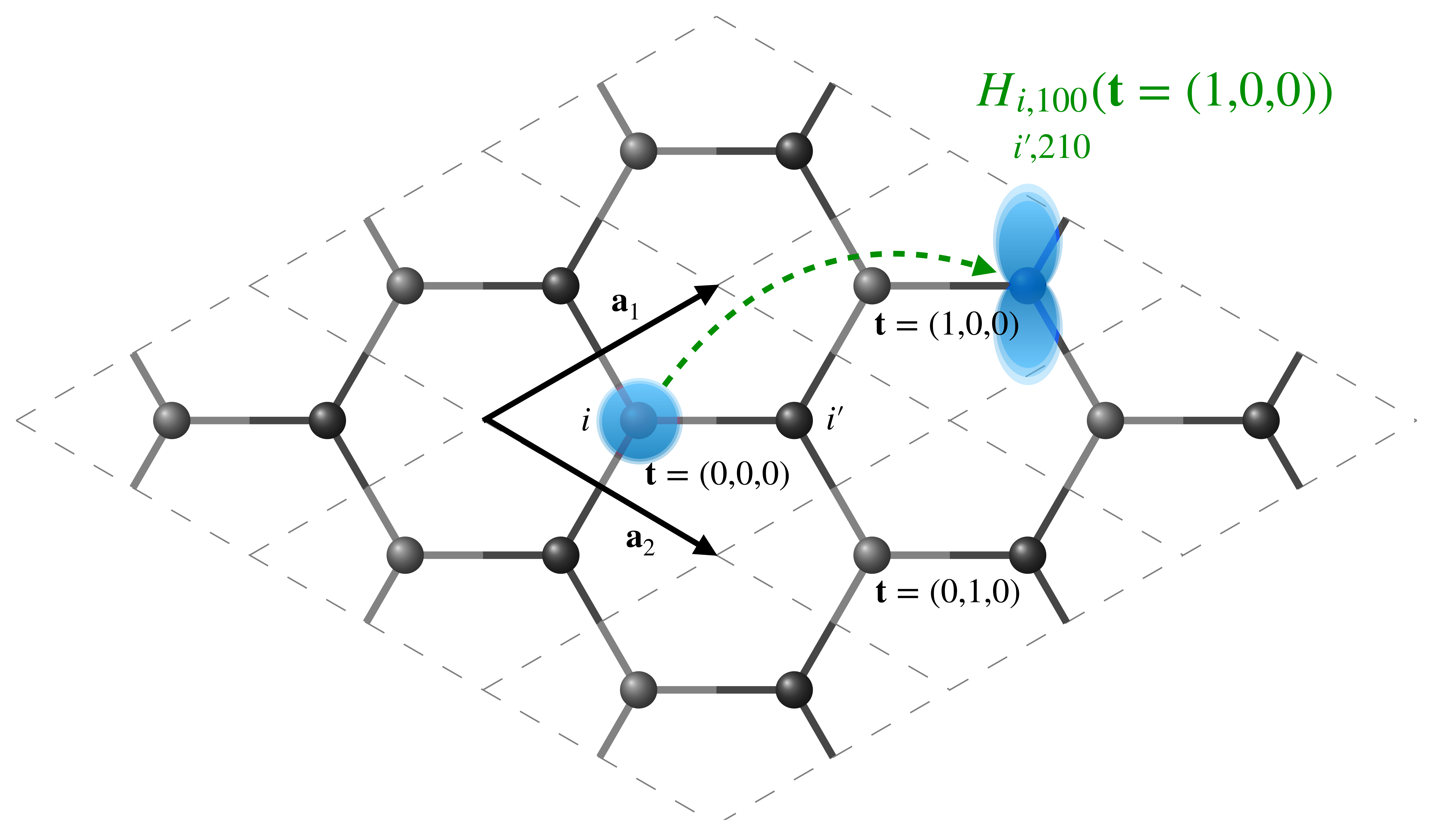
Representation of a graphene unit cell and its \(3 \times 3 \times 1\) replicas in real space. The central cell is denoted by \(\mathbf{t}=(0,0,0)\), while the cells translated by a single lattice vector along directions 1 and 2 are denoted by \(\mathbf{t}=(1,0,0)\) and \(\mathbf{t}=(0,1,0)\), respectively. The Hamiltonian matrix element between the \(1s\) orbital on atom \(i\) in the central unit cell and the \(2p_z\) orbital on atom \(i'\) in the \(\mathbf{t}=(1,0,0)\) cell is schematically represented.

Alternatively, we can provide the matrices in reciprocal (or Fourier, \(k\)) space. These are related to the real-space matrices by a Bloch sum,

\[\mathbf{H}(\mathbf{k})=\sum_{\mathbf{t}}\ e^{i\mathbf{k}\cdot\mathbf{t}} \mathbf{H}(\mathbf{t}).\]

In the case the input matrices are in reciprocal space, there should be one matrix per \(k\)-point in the grid.

A QMDataset to store the DFT data

The QMDataset class holds all the relevant data obtained from a quantum-mechanical (in this case, DFT) calculation, combining information from the files containing structures, Hamiltonians and overlap matrices, and \(k\)-point mesh.

qmdata = QMDataset.from_file(
    # File containing the atomistic structures
    frames_path="data/C2.xyz",
    # File containing the Hamiltonian (of Fock) matrices
    fock_realspace_path="graphene_fock.npy",
    # File containing the overlap matrices
    overlap_realspace_path="graphene_ovlp.npy",
    # File containing the k-point grids used for the DFT calculations
    kmesh_path="kmesh.dat",
    # Physical dimensionality of the system. Graphene is a 2D material
    dimension=2,
    # Device where to run the calculations
    # (can be 'cpu' or 'cuda', if GPUs are available)
    device="cpu",
    # Name of the basis set used for the calculations
    orbs_name=basis,
    # List of quantum numbers associated with the basis set orbitals
    orbs=orbitals[basis],
)

Quantities stored in QMDataset can be accessed as attributes, e.g. qmdata.fock_realspace is a list (one element per structure) of dictionaries labeled by the indices of the unit cell real-space translations containing torch.Tensor.

structure_idx = 0
realspace_translation = 0, 0, 0
print(f"The real-space Hamiltonian matrix for structure {structure_idx} labeled by")
print(f"translation T={realspace_translation} is:")
print(f"{qmdata.fock_realspace[structure_idx][realspace_translation]}")

The real-space Hamiltonian matrix for structure 0 labeled by
translation T=(0, 0, 0) is:
tensor([[-9.7210e+00, -2.6676e+00,  2.9317e-04,  3.2255e-04,  5.7009e-04,
         -8.1646e-05, -4.6611e-01, -3.6897e-01, -1.2792e-02,  6.7660e-01],
        [-2.6676e+00, -1.3880e+00,  3.2649e-03,  7.2985e-03,  1.0359e-02,
         -4.6611e-01, -5.9615e-01, -2.5023e-01, -8.9866e-03,  4.5874e-01],
        [ 2.9317e-04,  3.2649e-03, -4.2835e-01, -9.5326e-05, -1.2642e-02,
          3.6897e-01,  2.5023e-01, -1.0482e-01,  3.3322e-03, -1.6016e-01],
        [ 3.2255e-04,  7.2985e-03, -9.5326e-05, -1.4549e-01, -2.8526e-04,
          1.2792e-02,  8.9865e-03,  3.3322e-03, -1.4956e-01, -6.0943e-03],
        [ 5.7009e-04,  1.0359e-02, -1.2642e-02, -2.8526e-04, -4.4633e-01,
         -6.7660e-01, -4.5874e-01, -1.6016e-01, -6.0944e-03,  1.0121e-01],
        [-8.1646e-05, -4.6611e-01,  3.6897e-01,  1.2792e-02, -6.7660e-01,
         -9.7210e+00, -2.6676e+00, -2.9113e-04, -3.2414e-04, -5.7176e-04],
        [-4.6611e-01, -5.9615e-01,  2.5023e-01,  8.9865e-03, -4.5874e-01,
         -2.6676e+00, -1.3880e+00, -3.2673e-03, -7.2983e-03, -1.0360e-02],
        [-3.6897e-01, -2.5023e-01, -1.0482e-01,  3.3322e-03, -1.6016e-01,
         -2.9113e-04, -3.2673e-03, -4.2835e-01, -9.5331e-05, -1.2644e-02],
        [-1.2792e-02, -8.9866e-03,  3.3322e-03, -1.4956e-01, -6.0944e-03,
         -3.2414e-04, -7.2983e-03, -9.5331e-05, -1.4549e-01, -2.8525e-04],
        [ 6.7660e-01,  4.5874e-01, -1.6016e-01, -6.0943e-03,  1.0121e-01,
         -5.7176e-04, -1.0360e-02, -1.2644e-02, -2.8525e-04, -4.4633e-01]])

Machine learning data set

Symmetries of the Hamiltonian matrix

The data stored in QMDataset can be transformed into a format that is optimal for machine learning modeling by leveraging the underlying physical symmetries that characterize the atomistic structure, the basis set, and their associated matrices.

The Hamiltonian matrix is a complex learning target, indexed by two atoms and the orbitals centered on them. Each \(\mathbf{H}(\mathbf{k})\) is a Hermitian matrix, while in real space, periodicity introduces a symmetry over translation pairs such that \(\mathbf{H}(-\mathbf{t}) = \mathbf{H}(\mathbf{t})^\dagger\), where the dagger, \(\dagger\), denotes Hermitian conjugation.

To address the symmetries associated with swapping atomic indices or orbital labels, we divide the matrix into blocks labeled by pairs of atom types.

• block_type = 0, or on-site blocks, consist of elements corresponding to the interaction of orbitals on the same atom, \(i = i'\).

• block_type = 2, or cross-species blocks, consist of elements corresponding to orbitals centered on atoms of distinct species. Since the two atoms can be distinguished, they can be consistently arranged in a predetermined order.

• block_type = 1, -1, or same-species blocks, consist of elements corresponding to orbitals centered on distinct atoms of the same species. As these atoms are indistinguishable and cannot be ordered definitively, the pair must be symmetrized for permutations. We construct symmetric and antisymmetric combinations \((\mathbf{H}_{\small\substack{i,nlm\\i',n'l'm'}}(\mathbf{t})\pm\ \mathbf{H}_{\small\substack{i',nlm\\i,n'l'm'}}(\mathbf{-t}))\) that correspond to block_type \(+1\) and \(-1\), respectively.

Equivariant structure of the Hamiltonians

Even though the Hamiltonian operator under consideration is invariant, its representation transforms under the action of structural rotations and inversions due to the choice of the basis functions. Each of the blocks has elements of the form \(\langle\mathbf{0}inlm|\hat{H}|\mathbf{t}i'n'l'm'\rangle\), which are in an uncoupled representation and transform as a product of (real) spherical harmonics, \(Y_l^m \otimes Y_{l'}^{m'}\).

This product can be decomposed into a direct sum of irreducible representations (irreps) of \(\mathrm{SO(3)}\),

\[\lambda \mu:\lambda \in [|l_1-l_2|,l_1+l_2],\mu \in [-\lambda,\lambda],\]

which express the Hamiltonian blocks in terms of contributions that rotate independently and can be modeled using a feature that geometrically describes the pair of atoms under consideration and shares the same symmetry. We use the notation \(H_{ii';nn'll'}^{\lambda\mu}\) to indicate the elements of the Hamiltonian in this coupled basis.

The resulting irreps form a coupled representation, each of which transforms as a spherical harmonic \(Y^\mu_\lambda\) under \(\mathrm{SO(3)}\) rotations, but may exhibit more complex behavior under inversions. For example, spherical harmonics transform under inversion, \(\hat{i}\), as polar tensors:

\[\hat{i}Y^\mu_\lambda = (-1)^\lambda Y^\mu_\lambda.\]

Some of the coupled basis terms transform like \(Y^\mu_\lambda\), while others instead transform as pseudotensors,

\[\hat{i}H^{\lambda\mu}=(-1)^{\lambda+1}H^{\lambda\mu}\]

where we omit for simplicity the indices that are not directly associated with inversion and rotation symmetry. For more details about the block decomposition, please refer to Nigam et al., J. Chem. Phys. 156, 014115 (2022).

The following is an animation of a trajectory along a Lissajous curve in 3D space, alongside a colormap representing the values of the real-space Hamiltonian matrix elements of the graphene unit cell in a minimal STO-3G basis. From the animation, it is evident how invariant elements, such as those associated with interactions between \(s\) orbitals, do not change under structural rotations. On the other hand, interactions allowing for equivariant components, such as the \(s\)-\(p\) block, change under rotations.

image_files = sorted(
    [
        f"frames/{f}"
        for f in os.listdir("./frames")
        if f.startswith("rot_") and f.endswith(".png")
    ]
)
images = [mpimg.imread(img) for img in image_files]
fig, ax = plt.subplots()
img_display = ax.imshow(images[0])
ax.axis("off")


def update(frame):
    img_display.set_data(images[frame])
    return [img_display]


ani = FuncAnimation(fig, update, frames=len(images), interval=20, blit=True)

Once Loop Reflect

from IPython.display import HTML
HTML(ani.to_jshtml())

Mapping geometric features to Hamiltonian targets

Each Hamiltonian block obtained from the procedure described above can be modeled using symmetrized features.

Elements of block_type=0 are indexed by a single atom and are best described by a symmetrized atom-centered density correlation (ACDC), denoted by \(|\overline{\rho_{i}^{\otimes \nu}; \sigma; \lambda\mu }\rangle\), where \(\nu\) refers to the correlation (body)-order, and—just as for the blocks—\(\lambda \mu\) indicate the \(\mathrm{SO(3)}\) irrep to which the feature is symmetrized. The symbol \(\sigma\) denotes the inversion parity.

For other blocks, such as block_type=2, which explicitly reference two atoms, we use two-center ACDCs, \(|\overline{\rho_{ii'}^{\otimes \nu}; \lambda\mu }\rangle\).

For block_type=1, -1, we ensure equivariance with respect to atom index permutation by constructing symmetric and antisymmetric pair features: \((|\overline{\rho_{ii'}^{\otimes \nu};\lambda\mu }\rangle\pm\ |\overline{\rho_{i'i}^{\otimes \nu};\lambda\mu }\rangle)\).

The features are discretized on a basis of radial functions and spherical harmonics, and their performance may depend on the resolution of the functions included in the model. There are additional hyperparameters, such as the cutoff radius, which controls the extent of the atomic environment, and Gaussian widths. In the following, we allow for flexibility in discretizing the atom-centered and two-centered ACDCs by defining the hyperparameters for the single-center (SC) \(\lambda\)-SOAP and two-center (TC) ACDC descriptors.

The single and two-center descriptors have very similar hyperparameters, except for the cutoff radius, which is larger for the two-center descriptors to explicitly include distant pairs of atoms.

Note that the descriptors of pairs of atoms separated by distances greater than the cutoff radius are identically zero. Thus, any model based on these descriptors would predict an identically zero value for these pairs.

SC_HYPERS = {
    "cutoff": 3.0,
    "max_radial": 6,
    "max_angular": 6,
    "atomic_gaussian_width": 0.5,
    "center_atom_weight": 1,
    "radial_basis": {"Gto": {}},
    "cutoff_function": {"ShiftedCosine": {"width": 0.5}},
}

TC_HYPERS = {
    "cutoff": 6.0,
    "max_radial": 6,
    "max_angular": 6,
    "atomic_gaussian_width": 0.3,
    "center_atom_weight": 1.0,
    "radial_basis": {"Gto": {}},
    "cutoff_function": {"ShiftedCosine": {"width": 0.5}},
}

We then use the above defined hyperparameters to compute the descriptor and initialize a MLDataset instance, which contains, among other things, the Hamiltonian block decomposition and the geometric features described above.

In addition to computing the descriptors, MLDataset takes the data stored in the QMDataset instance and puts it in a form required to train a ML model.

The item_names argument is a list of names of the quantities we want to compute and target in the ML model training, or that we want to be able to access later.

For example, fock_blocks is a metatensor.Tensormap containing the Hamiltonian coupled blocks. We also want to access the overlap matrices in \(k\)-space (overlap_kspace) to be able to compute the Hamiltonian eigenvalues in the \(k\)-grid.

mldata = MLDataset(
    # A QMDataset instance
    qmdata,
    # The names of the quantities to compute/initialize for the training
    item_names=["fock_blocks", "overlap_kspace"],
    # Hypers for the SC descriptors
    hypers_atom=SC_HYPERS,
    # Hypers for the TC descriptors
    hypers_pair=TC_HYPERS,
    # Cutoff for the angular quantum number to use in the Clebsh-Gordan iterations
    lcut=4,
    # Fraction of structures in the training set
    train_frac=0.7,
    # Fraction of structures in the validation set
    val_frac=0.2,
    # Fraction of structures in the test set
    test_frac=0.1,
    # Whether to shuffle or not the structure indices before splitting the data set
    shuffle=True,
)

cpu pair features
cpu single center features
cpu single center features

The matrix decomposition into blocks and the calculations of geometric features is performed by the MLDataset class.

mldata.features is metatensor.TensorMap containing the stuctures’ descriptors

mldata.features

TensorMap with 27 blocks
keys: order_nu  inversion_sigma  spherical_harmonics_l  species_center  species_neighbor  block_type
         2            -1                   1                  6                6              -1
         2            -1                   1                  6                6              0
         2            -1                   1                  6                6              1
         2            -1                   2                  6                6              -1
         2            -1                   2                  6                6              0
         2            -1                   2                  6                6              1
         2            -1                   3                  6                6              -1
         2            -1                   3                  6                6              0
         2            -1                   3                  6                6              1
         2            -1                   4                  6                6              -1
         2            -1                   4                  6                6              0
         2            -1                   4                  6                6              1
         2             1                   0                  6                6              -1
         2             1                   0                  6                6              0
         2             1                   0                  6                6              1
         2             1                   1                  6                6              -1
         2             1                   1                  6                6              0
         2             1                   1                  6                6              1
         2             1                   2                  6                6              -1
         2             1                   2                  6                6              0
         2             1                   2                  6                6              1
         2             1                   3                  6                6              -1
         2             1                   3                  6                6              0
         2             1                   3                  6                6              1
         2             1                   4                  6                6              -1
         2             1                   4                  6                6              0
         2             1                   4                  6                6              1

mldata.items is a namedtuple containing the quantities defined in item_names. e.g. the coupled Hamiltonian blocks:

print("The TensorMap containing the Hamiltonian coupled blocks is")
mldata.items.fock_blocks

The TensorMap containing the Hamiltonian coupled blocks is

TensorMap with 9 blocks
keys: block_type  species_i  species_j  L  inversion_sigma
          -1          6          6      0         1
          -1          6          6      1        -1
          -1          6          6      1         1
          0           6          6      0         1
          0           6          6      1         1
          0           6          6      2         1
          1           6          6      0         1
          1           6          6      1         1
          1           6          6      2         1

Or the overlap matrices:

structure_idx = 0
k_idx = 0
print(f"The overlap matrix for structure {structure_idx} at the {k_idx}-th k-point is")
mldata.items.overlap_kspace[structure_idx][k_idx]

The overlap matrix for structure 0 at the 0-th k-point is

tensor([[ 1.0000e+00+0.j,  2.6471e-01+0.j, -8.6736e-19+0.j, -3.4717e-16+0.j,
          0.0000e+00+0.j,  8.4955e-06+0.j,  1.3441e-01+0.j,  8.8189e-04+0.j,
          3.7267e-03+0.j,  3.8015e-03+0.j],
        [ 2.6471e-01+0.j,  1.4675e+00+0.j,  5.4607e-25+0.j, -2.2147e-16+0.j,
          2.6503e-23+0.j,  1.3441e-01+0.j,  1.3276e+00+0.j, -7.6212e-04+0.j,
          2.2394e-02+0.j,  4.7228e-03+0.j],
        [ 8.6736e-19+0.j, -5.4607e-25+0.j,  6.5783e-01+0.j,  6.3610e-17+0.j,
          6.2688e-04+0.j, -8.8189e-04+0.j,  7.6212e-04+0.j, -2.4925e-01+0.j,
         -2.1836e-05+0.j, -1.6848e-02+0.j],
        [ 3.4717e-16+0.j,  2.2147e-16+0.j,  6.3610e-17+0.j,  1.2005e+00+0.j,
          3.4697e-17+0.j, -3.7267e-03+0.j, -2.2394e-02+0.j, -2.1836e-05+0.j,
          7.7122e-01+0.j, -2.4677e-04+0.j],
        [ 0.0000e+00+0.j, -2.6503e-23+0.j,  6.2688e-04+0.j,  3.4697e-17+0.j,
          6.6397e-01+0.j, -3.8015e-03+0.j, -4.7228e-03+0.j, -1.6848e-02+0.j,
         -2.4677e-04+0.j, -2.7830e-01+0.j],
        [ 8.4955e-06+0.j,  1.3441e-01+0.j, -8.8189e-04+0.j, -3.7267e-03+0.j,
         -3.8015e-03+0.j,  1.0000e+00+0.j,  2.6471e-01+0.j,  0.0000e+00+0.j,
          0.0000e+00+0.j,  0.0000e+00+0.j],
        [ 1.3441e-01+0.j,  1.3276e+00+0.j,  7.6212e-04+0.j, -2.2394e-02+0.j,
         -4.7228e-03+0.j,  2.6471e-01+0.j,  1.4675e+00+0.j,  5.4607e-25+0.j,
          0.0000e+00+0.j,  2.6501e-23+0.j],
        [ 8.8189e-04+0.j, -7.6212e-04+0.j, -2.4925e-01+0.j, -2.1836e-05+0.j,
         -1.6848e-02+0.j,  0.0000e+00+0.j, -5.4607e-25+0.j,  6.5783e-01+0.j,
          0.0000e+00+0.j,  6.2688e-04+0.j],
        [ 3.7267e-03+0.j,  2.2394e-02+0.j, -2.1836e-05+0.j,  7.7122e-01+0.j,
         -2.4677e-04+0.j,  0.0000e+00+0.j,  0.0000e+00+0.j,  0.0000e+00+0.j,
          1.2005e+00+0.j,  0.0000e+00+0.j],
        [ 3.8015e-03+0.j,  4.7228e-03+0.j, -1.6848e-02+0.j, -2.4677e-04+0.j,
         -2.7830e-01+0.j,  0.0000e+00+0.j, -2.6501e-23+0.j,  6.2688e-04+0.j,
          0.0000e+00+0.j,  6.6397e-01+0.j]])

A machine learning model for the electronic Hamiltonian of graphene

Linear model

In simple cases, such as the present one, it is convenient to start with a linear model that directly maps the geometric descriptors to the target coupled blocks. This can be achieved using Ridge regression as implemented in scikit-learn.

The linear regression model is expressed as

\[H_{ii',\mathbf{Q}}^{\lambda\mu}(\mathbf{t}) = \ \sum_\mathbf{q} w_{\mathbf{q}}^{\mathbf{Q},\lambda} \ (\rho_{ii'}^{\otimes \nu}(\mathbf{t}))_{\mathbf{q}}^{\lambda\mu},\]

where a shorthand notation for the features has been introduced. Here, \(\mathbf{Q}\) includes all labels indicating the involved orbitals, atomic species, and permutation symmetry, while \(\mathbf{q}\) represents the feature dimension. The quantities \(w_{\mathbf{q}}^{\mathbf{Q},\lambda}\) are the model’s weights. Note that different weights are associated with different values of \(\mathbf{Q}\) and \(\lambda\), but not with specific atom pairs or the translation vector, whose dependence arises only through the descriptors.

In mlelec, a linear model can be trained through the LitEquivariantModel class, which accepts an init_from_ridge keyword. When set to True, this initializes the weights of a more general torch.nn.Module with the weights provided by Ridge regression.

We will pass other keyword arguments to LitEquivariantModel, to be able to further train the weights on top to the initial Ridge regression.

model = LitEquivariantModel(
    mldata=mldata,  # a MLDataset instance
    nlayers=0,  # The number of hidden layers
    nhidden=1,  # The number of neurons in each hidden layer
    init_from_ridge=True,  # If True, initialize the weights and biases of the
    # purely linear model from Ridge regression
    optimizer="LBFGS",  # Type of optimizer. Adam is likely better for
    # a more general neural network
    activation="SiLU",  # The nonlinear activation function
    learning_rate=1e-3,  # Initial learning rate (LR)
    lr_scheduler_patience=10,
    lr_scheduler_factor=0.7,
    lr_scheduler_min_lr=1e-6,
    loss_fn=MSELoss(),  # Use the mean square error as loss function
)

Model’s accuracy in reproducing derived properties

The Hamiltonian coupled blocks predicted by the ML model can be accessed from model.forward()

predicted_blocks = model.forward(mldata.features)

The real-space blocks can be transformed to Hamiltonian matrices via the mlelec.utils.pbc_utils.blocks_to_matrix function. The resulting real-space Hamiltonians can be Fourier transformed to give the \(k\)-space ones.

HT = blocks_to_matrix(
    predicted_blocks,
    orbitals["sto-3g"],
    {A: qmdata.structures[A] for A in range(len(qmdata))},
    detach=True,
)
Hk = qmdata.bloch_sum(HT, is_tensor=True)

Kohn-Sham eigenvalues

We can then compute the eigenvalues on the \(k\)-grid used for the calculation to assess the model accuracy in predicting band energies.

target_eigenvalues = compute_eigenvalues(qmdata.fock_kspace, qmdata.overlap_kspace)
predicted_eigenvalues = compute_eigenvalues(Hk, qmdata.overlap_kspace)

Hartree = 27.211386024367243  # eV

plt.rcParams["font.size"] = 14
fig, ax = plt.subplots()
ax.set_aspect("equal")

x_text = 0.38
y_text = 0.2
d = 0.06

for i, (idx, label) in enumerate(
    zip(
        [mldata.train_idx, mldata.val_idx, mldata.test_idx],
        ["train", "validation", "test"],
    )
):

    target = (
        torch.stack([target_eigenvalues[i] for i in idx]).flatten().detach() * Hartree
    )
    prediction = (
        torch.stack([predicted_eigenvalues[i] for i in idx]).flatten().detach()
        * Hartree
    )

    non_core_states = target > -100
    rmse = np.sqrt(
        np.mean(
            (target.numpy()[non_core_states] - prediction.numpy()[non_core_states]) ** 2
        )
    )
    ax.scatter(target, prediction, marker=".", label=label, alpha=0.5)
    ax.text(
        x=x_text,
        y=y_text - d * i,
        s=rf"$\mathrm{{RMSE_{{{label}}}={rmse:.2f}\,eV}}$",
        transform=ax.transAxes,
    )

xmin, xmax = ax.get_xlim()
ax.plot([xmin, xmax], [xmin, xmax], "--k")
ax.set_xlim(xmin, xmax)
ax.set_ylim(xmin, xmax)
ax.legend()
ax.set_xlabel("Target eigenvalues (eV)")
ax.set_ylabel("Predicted eigenvalues (eV)")

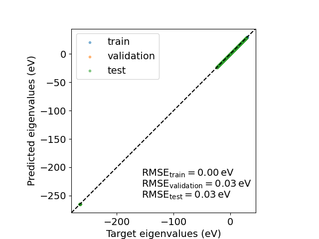
Text(74.4222222222222, 0.5, 'Predicted eigenvalues (eV)')

Graphene band structure

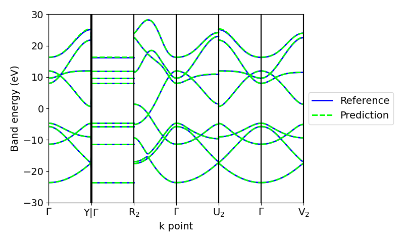
Apart from the eigenvalues on a mesh in the Brillouin zone, we can use the real-space Hamiltonians predicted by the model to compute the band structure along high-symmetry paths.

fig, ax = plt.subplots(figsize=(8, 4.8))

idx = 0

handles = []

with warnings.catch_warnings():
    warnings.filterwarnings("ignore", category=DeprecationWarning)

    # Plot reference
    ax, h_ref = plot_bands_frame(
        qmdata.fock_realspace[idx], idx, qmdata, ax=ax, color="blue", lw=2
    )

    # Plot prediction
    ax, h_pred = plot_bands_frame(
        HT[idx], idx, qmdata, ax=ax, color="lime", ls="--", lw=2
    )

ax.set_ylim(-30, 30)
ax.legend(
    [h_ref, h_pred],
    ["Reference", "Prediction"],
    loc="center left",
    bbox_to_anchor=(1, 0.5),
)
fig.tight_layout()

/home/runner/work/atomistic-cookbook/atomistic-cookbook/.nox/periodic-hamiltonian/lib/python3.11/site-packages/spglib/spglib.py:115: DeprecationWarning: dict interface (SpglibDataset['std_lattice']) is deprecated.Use attribute interface ({self.__class__.__name__}.{key}) instead
  warnings.warn(
/home/runner/work/atomistic-cookbook/atomistic-cookbook/.nox/periodic-hamiltonian/lib/python3.11/site-packages/spglib/spglib.py:115: DeprecationWarning: dict interface (SpglibDataset['std_positions']) is deprecated.Use attribute interface ({self.__class__.__name__}.{key}) instead
  warnings.warn(
/home/runner/work/atomistic-cookbook/atomistic-cookbook/.nox/periodic-hamiltonian/lib/python3.11/site-packages/spglib/spglib.py:115: DeprecationWarning: dict interface (SpglibDataset['std_types']) is deprecated.Use attribute interface ({self.__class__.__name__}.{key}) instead
  warnings.warn(
/home/runner/work/atomistic-cookbook/atomistic-cookbook/.nox/periodic-hamiltonian/lib/python3.11/site-packages/spglib/spglib.py:115: DeprecationWarning: dict interface (SpglibDataset['number']) is deprecated.Use attribute interface ({self.__class__.__name__}.{key}) instead
  warnings.warn(
/home/runner/work/atomistic-cookbook/atomistic-cookbook/.nox/periodic-hamiltonian/lib/python3.11/site-packages/spglib/spglib.py:115: DeprecationWarning: dict interface (SpglibDataset['transformation_matrix']) is deprecated.Use attribute interface ({self.__class__.__name__}.{key}) instead
  warnings.warn(
/home/runner/work/atomistic-cookbook/atomistic-cookbook/.nox/periodic-hamiltonian/lib/python3.11/site-packages/spglib/spglib.py:115: DeprecationWarning: dict interface (SpglibDataset['international']) is deprecated.Use attribute interface ({self.__class__.__name__}.{key}) instead
  warnings.warn(
/home/runner/work/atomistic-cookbook/atomistic-cookbook/.nox/periodic-hamiltonian/lib/python3.11/site-packages/spglib/spglib.py:115: DeprecationWarning: dict interface (SpglibDataset['std_rotation_matrix']) is deprecated.Use attribute interface ({self.__class__.__name__}.{key}) instead
  warnings.warn(
/home/runner/work/atomistic-cookbook/atomistic-cookbook/.nox/periodic-hamiltonian/lib/python3.11/site-packages/spglib/spglib.py:115: DeprecationWarning: dict interface (SpglibDataset['std_lattice']) is deprecated.Use attribute interface ({self.__class__.__name__}.{key}) instead
  warnings.warn(
/home/runner/work/atomistic-cookbook/atomistic-cookbook/.nox/periodic-hamiltonian/lib/python3.11/site-packages/spglib/spglib.py:115: DeprecationWarning: dict interface (SpglibDataset['std_positions']) is deprecated.Use attribute interface ({self.__class__.__name__}.{key}) instead
  warnings.warn(
/home/runner/work/atomistic-cookbook/atomistic-cookbook/.nox/periodic-hamiltonian/lib/python3.11/site-packages/spglib/spglib.py:115: DeprecationWarning: dict interface (SpglibDataset['std_types']) is deprecated.Use attribute interface ({self.__class__.__name__}.{key}) instead
  warnings.warn(
/home/runner/work/atomistic-cookbook/atomistic-cookbook/.nox/periodic-hamiltonian/lib/python3.11/site-packages/spglib/spglib.py:115: DeprecationWarning: dict interface (SpglibDataset['number']) is deprecated.Use attribute interface ({self.__class__.__name__}.{key}) instead
  warnings.warn(
/home/runner/work/atomistic-cookbook/atomistic-cookbook/.nox/periodic-hamiltonian/lib/python3.11/site-packages/spglib/spglib.py:115: DeprecationWarning: dict interface (SpglibDataset['transformation_matrix']) is deprecated.Use attribute interface ({self.__class__.__name__}.{key}) instead
  warnings.warn(
/home/runner/work/atomistic-cookbook/atomistic-cookbook/.nox/periodic-hamiltonian/lib/python3.11/site-packages/spglib/spglib.py:115: DeprecationWarning: dict interface (SpglibDataset['international']) is deprecated.Use attribute interface ({self.__class__.__name__}.{key}) instead
  warnings.warn(
/home/runner/work/atomistic-cookbook/atomistic-cookbook/.nox/periodic-hamiltonian/lib/python3.11/site-packages/spglib/spglib.py:115: DeprecationWarning: dict interface (SpglibDataset['std_rotation_matrix']) is deprecated.Use attribute interface ({self.__class__.__name__}.{key}) instead
  warnings.warn(

Adding nonlinearities

The model used above consists of several submodels, one for each Hamiltonian coupled block. Each submodel can be extended to a multilayer perceptron (MLP) that maps the corresponding set of geometric features to the Hamiltonian coupled block. Nonlinearities are applied to the invariants constructed from each equivariant feature block using the EquivariantNonlinearity module. This section outlines the process to modify the model to introduce non-linear terms. Given that the time to train and evaluate the model would then increase, this section includes snippets of code, but is not a complete implementation and is not executed when running this example.

The architecture of EquivariantNonlinearity can be visualized with torchviz with the following snippet:

import torch
from mlelec.models.equivariant_model import EquivariantNonLinearity
from torchviz import make_dot
m = EquivariantNonLinearity(torch.nn.SiLU(), layersize = 10)
y = m.forward(torch.randn(3,3,10))
dot = make_dot(y, dict(m.named_parameters()))
dot.graph_attr.update(size='150,150')
dot.render("equivariantnonlinear", format="png")
dot

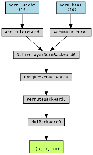
Graph representing the architecture of EquivariantNonLinearity

The global architecture of the MLP, implemented in simpleMLP, can be visualized with

import torch
from mlelec.models.equivariant_model import simpleMLP
from torchviz import make_dot
mlp = simpleMLP(
    nin=10,
    nout=1,
    nhidden=1,
    nlayers=1,
    bias=True,
    activation='SiLU',
    apply_layer_norm=True
    )
y = mlp.forward(torch.randn(1,1,10))
dot = make_dot(y, dict(mlp.named_parameters()))
dot.graph_attr.update(size='150,150')
dot.render("simpleMLP", format="png")
dot

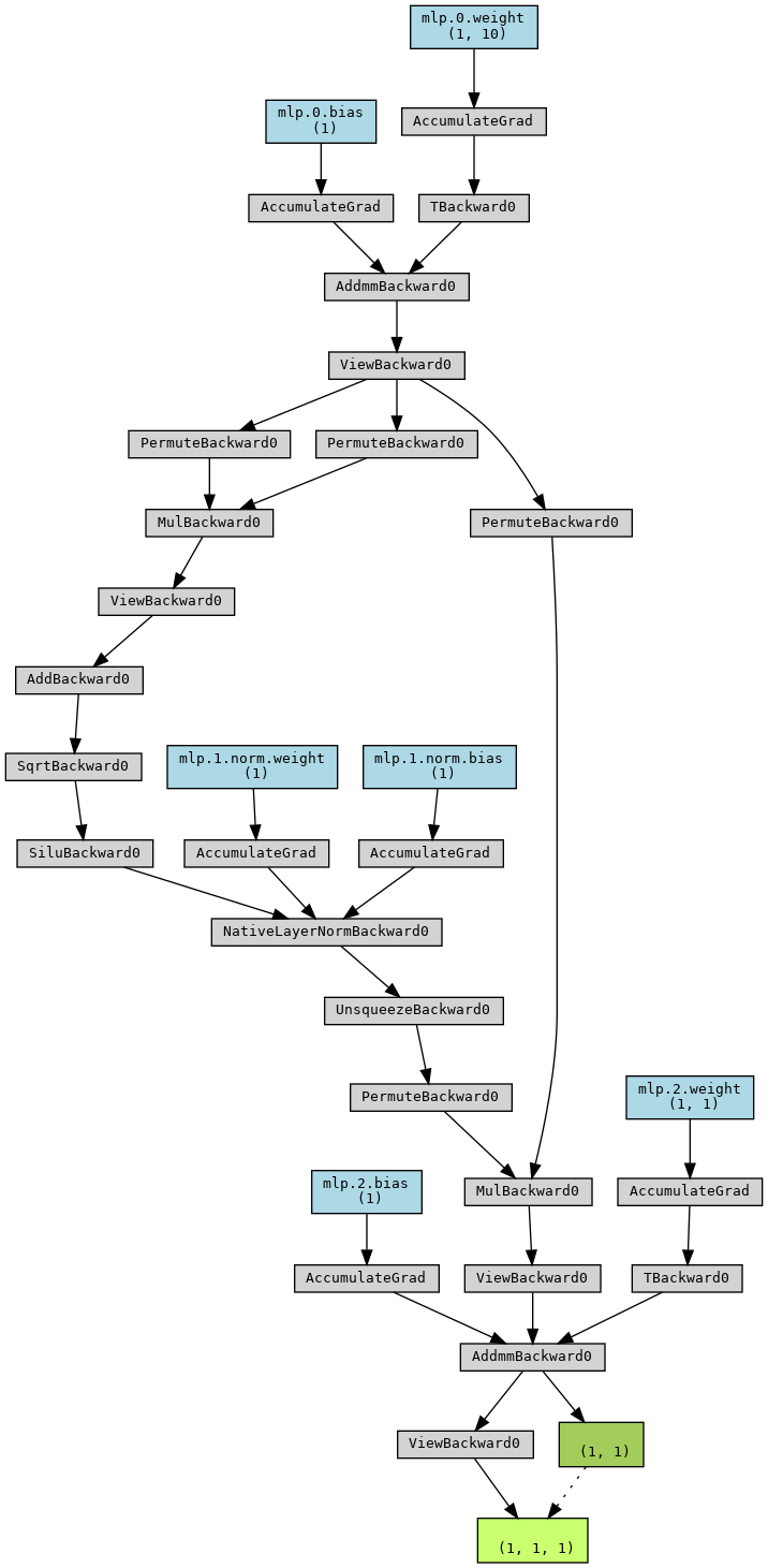
Graph representing the architecture of simpleMLP

Import additional modules needed to monitor the training.

import lightning.pytorch as pl
from lightning.pytorch.callbacks import EarlyStopping
from mlelec.callbacks.logging import LoggingCallback
from mlelec.models.equivariant_lightning import MLDatasetDataModule

We set up a callback for logging training information such as the training and validation losses.

logger_callback = LoggingCallback(log_every_n_epochs=5)

We set up an early stopping criterion to stop the training when the validation loss function stops decreasing.

early_stopping = EarlyStopping(
    monitor="val_loss", min_delta=1e-3, patience=10, verbose=False, mode="min"
)

We define a lighting.pytorch.Trainer instance to handle the training loop. For example, we can further optimize the weights for 50 epochs using the LBFGS optimizer.

Note that PyTorch Lightning requires the definition of a data module to instantiate DataLoaders to be used during the training.

data_module = MLDatasetDataModule(mldata, batch_size=16, num_workers=0)

trainer = pl.Trainer(
    max_epochs=50,
    accelerator="cpu",
    check_val_every_n_epoch=10,
    callbacks=[early_stopping, logger_callback],
    logger=False,
    enable_checkpointing=False,
)

trainer.fit(model, data_module)

We compute the test set loss to assess the model accuracy on an unseen set of structures

trainer.test(model, data_module)

In this case, Ridge regression already provides good accuracy, so further optimizing the weights offers limited improvement. However, for more complex datasets, the benefits of additional optimization can be significant.