LPR analysis for amorphous silicon dataset

Authors:

Sanggyu “Raymond” Chong @SanggyuChong; Federico Grasselli @fgrassel

In this tutorial, we calculate the SOAP descriptors of an amorphous silicon dataset using rascaline, then compute the local prediction rigidity (LPR) for the atoms of a “test” set before and after modifications to the “training” dataset has been made.

First, we import all the necessary packages:

import os
import tarfile

import numpy as np
import requests
from ase.io import read
from matplotlib import pyplot as plt
from matplotlib.colors import LogNorm
from rascaline import SoapPowerSpectrum
from sklearn.decomposition import PCA
from skmatter.metrics import local_prediction_rigidity as lpr

Load and prepare amorphous silicon data

We first download the dataset associated with LPR analysis from Materials Cloud and load the the amorphous silicon structures using ASE.

filename = "LPR_supp_notebook_dataset.tar.gz"
if not os.path.exists(filename):
    url = "https://rb.gy/wxsrug"  # shortened URL
    response = requests.get(url)
    response.raise_for_status()
    with open(filename, "wb") as f:
        f.write(response.content)

with tarfile.open(filename) as tar:
    tar.extractall(path=".")

frames_pristine = read("datasets/Si_amo_defect_free.xyz", ":")
frames_defect = read("datasets/Si_amo_defect_containing.xyz", ":")

# Randomly shuffle the structures

np.random.seed(20230215)

ids = list(range(len(frames_pristine)))
np.random.shuffle(ids)
frames_pristine = [frames_pristine[ii] for ii in ids]

ids = list(range(len(frames_defect)))
np.random.shuffle(ids)
frames_defect = [frames_defect[ii] for ii in ids]

We now further refine the loaded datasets according the the number of coordinated atoms that each atomic environment exhibits. “Pristine” refers to structures where all of the atoms have strictly 4 coordinating atoms. “Defect” refers to structures that contain atoms with coordination numbers other than 4.

We use get_all_distances funciton of ase.Atoms to detect the number of coordinated atoms.

cur_cutoff = 2.7
refined_pristine_frames = []
for frame in frames_pristine:
    neighs = (frame.get_all_distances(mic=True) < cur_cutoff).sum(axis=0) - 1
    if neighs.max() > 4 or neighs.min() < 4:
        continue
    else:
        refined_pristine_frames.append(frame)

refined_defect_frames = []
for frame in frames_defect:
    neighs = (frame.get_all_distances(mic=True) < cur_cutoff).sum(axis=0) - 1
    num_defects = (neighs > 4).sum() + (neighs < 4).sum()
    if num_defects > 4:
        refined_defect_frames.append(frame)

Compute SOAP descriptors using rascaline

Now, we move on and compute the SOAP descriptors for the refined structures. First, define the rascaline hyperparameters used to compute SOAP. Among the hypers, notice that the cutoff is chosen to be 2.85 Å, and the radial scaling is turned off. These were heuristic choices made to accentuate the difference in the LPR based on the nearest-neighbor coordination. (Do not blindly use this set of hypers for production-quality model training!)

# Hypers dictionary
hypers = {
    "cutoff": 2.85,
    "max_radial": 10,
    "max_angular": 12,
    "atomic_gaussian_width": 0.5,
    "center_atom_weight": 1.0,
    "radial_basis": {"Gto": {"spline_accuracy": 1e-8}},
    "cutoff_function": {"ShiftedCosine": {"width": 0.1}},
    "radial_scaling": None,
}
# Define rascaline calculator
calculator = SoapPowerSpectrum(**hypers)

# Calculate the SOAP power spectrum
Xlist_pristine = []
for frame in refined_pristine_frames:
    descriptor = calculator.compute(frame)
    Xlist_pristine.append(np.array(descriptor.block().values))

Xlist_defect = []
for frame in refined_defect_frames:
    descriptor = calculator.compute(frame)
    Xlist_defect.append(np.array(descriptor.block().values))

Organize structures into “training” and “test” sets

Now we move on and compute the SOAP descriptors for the refined structures. First, define the rascaline hyperparameters used to compute SOAP.

Notice that the format in which we handle the descriptors is as a list of np.array descriptor blocks. This is to ensure compatibility with how things have been implemented in the LPR module of scikit-matter.

n_train = 400
n_add = 50
n_test = 50

X_pristine = [Xlist for Xlist in Xlist_pristine[: n_train + n_add]]
X_defect = [Xlist for Xlist in Xlist_defect[:n_add]]
X_test = [Xlist for Xlist in Xlist_defect[n_add : n_add + n_test]]

# Save coordination values for visualization
test_coord = []
for frame in refined_defect_frames[n_add : n_add + n_test]:
    coord = (frame.get_all_distances(mic=True) < cur_cutoff - 0.05).sum(axis=0) - 1
    test_coord += coord.tolist()
test_coord = np.array(test_coord)

Compute the LPR for the test set

Next, we will use the local_prediction_rigidity module of scikit-matter to compute the LPRs for the test set that we have set apart.

LPR reflects how the ML model perceives a local environment, given a collection of other structures, similar or different. It should then carry over some of the details involved in training the model, in this case the regularization strength.

For this example, we have foregone on the actual model training, and so we define an arbitrary value for the alpha.

alpha = 1e-4
LPR_test, rank = lpr(X_pristine, X_test, alpha)
LPR_test = np.hstack(LPR_test)

Visualizing the LPR on a PCA map

We now visualize the LPRs of the test set on a PCA map, where the PCA is performed on the SOAP descriptors of defect-containing dataset.

pca = PCA(n_components=5)
descriptors_all = calculator.compute(refined_defect_frames)
pca.fit_transform(descriptors_all.block().values)
PCA_test = pca.transform(np.vstack(X_test))

rmin = np.log10(LPR_test.min()) + 0.5
rmax = np.log10(LPR_test.max()) - 0.5

fig = plt.figure(figsize=(5, 4), dpi=200)
ax = fig.add_subplot()
im = ax.scatter(
    PCA_test[:, 0],
    PCA_test[:, 1],
    c=LPR_test,
    s=20,
    linewidths=0,
    norm=LogNorm(vmin=10**rmin, vmax=10**rmax),
    cmap="viridis",
)

ax.set_xlabel("PC1")
ax.set_ylabel("PC2")
fig.colorbar(im, ax=ax, label="LPR")
ax.tick_params(left=False, bottom=False, labelleft=False, labelbottom=False)
plt.show()

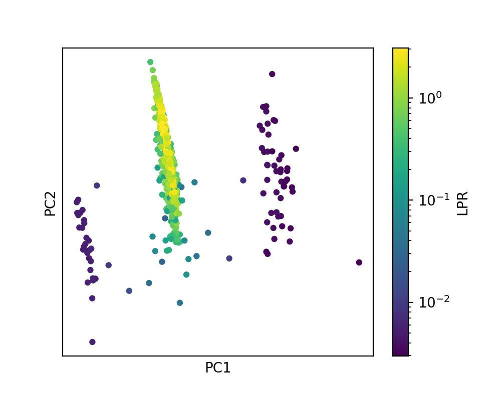
In the PCA map, where each point corresponds to an atomic environment of the test set structures, one can observe 4 different clusters of points, arranged along PC1. This corresponds to the coordination numbers ranging from 3 to 6. Since the training set contains structures exclusively composed of 4-coordinated atoms, LPR is distinctly high for the second, main cluster of points, and quite low for the three other clusters.

Studying the LPR after dataset modification

We now want to see what would happen when defect structures are included into the training set of the model. For this, we first create a modified dataset that incorporates in the defect structures, and recompute the LPR.

X_new = X_pristine[:n_train] + X_defect[:n_add]
LPR_test_new, rank = lpr(X_new, X_test, alpha)
LPR_test_new = np.hstack(LPR_test_new)

We then visualize the change in the LPR with the modification of the dataset by plotting the same PCA map, but now colored by the ratio of new set of LPR values (after dataset modification) over the original one.

fig = plt.figure(figsize=(5, 4), dpi=200)
ax = fig.add_subplot()
im = ax.scatter(
    PCA_test[:, 0],
    PCA_test[:, 1],
    c=LPR_test_new / LPR_test,
    s=20,
    linewidths=0,
    # norm=LogNorm(vmin=10**rmin, vmax=10**rmax),
    cmap="OrRd",
)
ax.set_xlabel("PC1")
ax.set_ylabel("PC2")
fig.colorbar(im, ax=ax, label=r"LPR$_{\mathrm{new}}$ / LPR$_{\mathrm{old}}$")
ax.tick_params(left=False, bottom=False, labelleft=False, labelbottom=False)
plt.show()

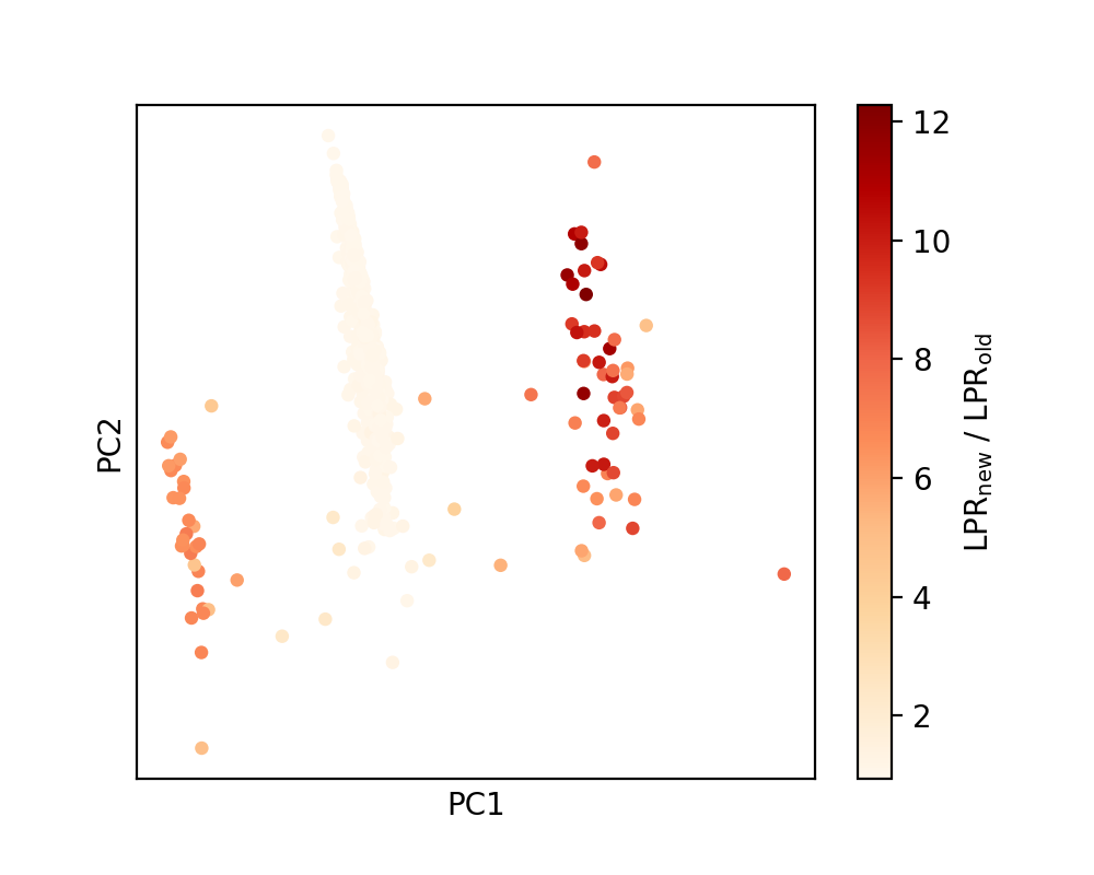
It is apparent that while the LPR stays more or less consistent for the 4-coordinated atoms, it is significantly enhanced for the defective environments as a result of the inclusion of defective structures in the training set.