Path integral metadynamics

Authors:

Michele Ceriotti @ceriottm

This example shows how to run a free-energy sampling calculation that combines path integral molecular dynamics to model nuclear quantum effects and metadynamics to accelerate sampling of the high-free-energy regions.

The rather complicated setup combines i-PI to perform path integral MD, its built-in driver to compute energy and forces for the Zundel \(\mathrm{H_5O_2^+}\) cation, and PLUMED to perform metadynamics. If you want to see an example in a more realistic scenario, you can look at this paper (Rossi et al., JCTC (2020)), in which this methodology is used to simulate the decomposition of methanesulphonic acid in a solution of phenol and hydrogen peroxide.

Note also that, in order to keep the execution time of this example as low as possible, several parameters are set to values that would not be suitable for an accurate, converged simulation. They will be highlighted and more reasonable values will be provided. “High-quality” runs can also be realized substituting the input files used in this example with those labeled with the _hiq suffix, that are also provided in the data/ folder.

import bz2
import os
import subprocess
import time
import xml.etree.ElementTree as ET

import ase
import ase.io
import chemiscope
import ipi
import matplotlib.pyplot as plt
import numpy as np

Metadynamics for the Zundel cation

Metadynamics is a method to accelerate sampling of rare events - microscopic processes that are too infrequent to be observed over the time scale (ns-µs) accessible to molecular dynamics simulations. You can read one of the many excellent reviews on metadynamics (see e.g. Bussi and Branduardi (2015)), or follow a lecture from the PLUMED masterclass. In short, during a metadynamics simulation an adaptive biasing potential is built as a superimposition of Gaussians centered over configurations that have been previously visited by the trajectory. This discourages the system from remaining in high-probability configurations and accelerates sampling of free-energy barriers.

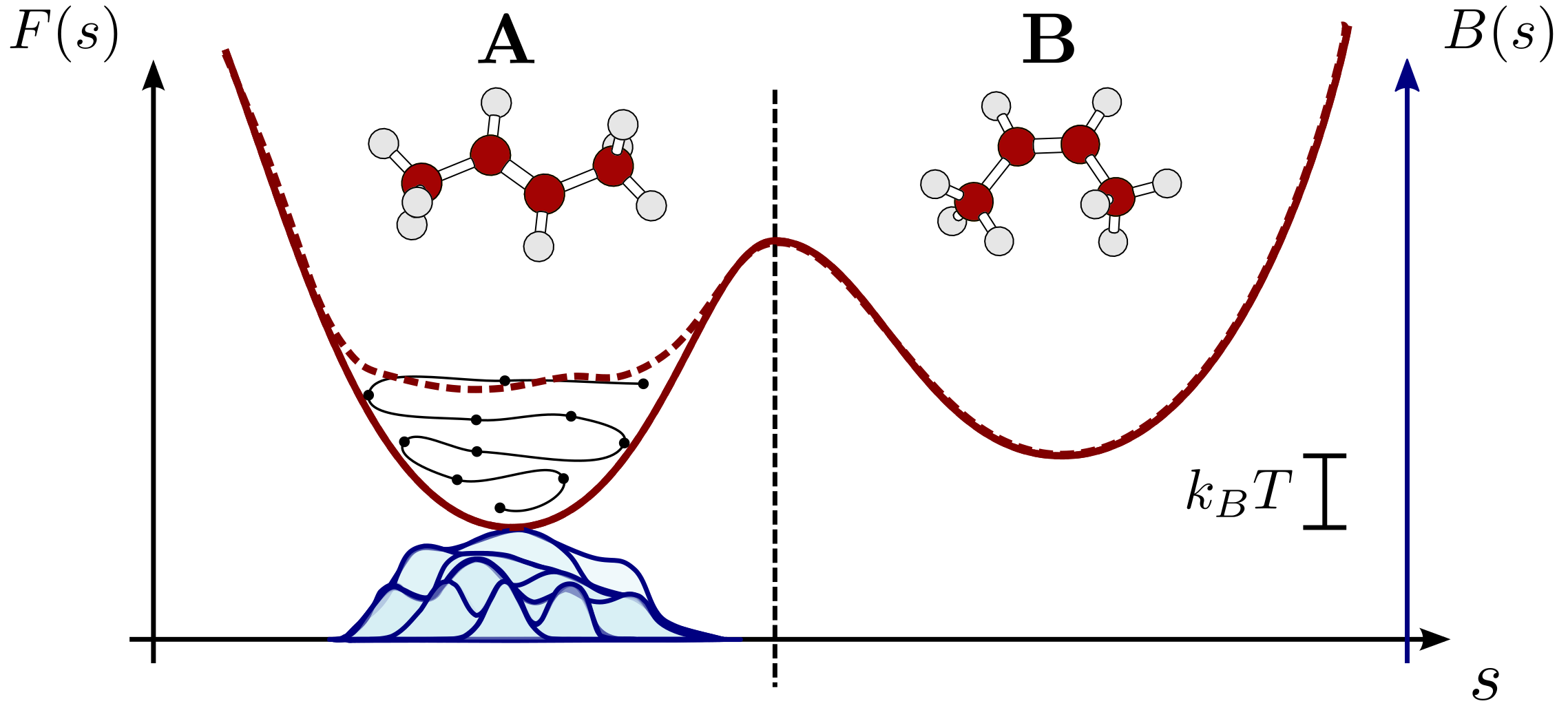
A schematic representation of how metadynamics work by adaptively building a repulsive bias based on the trajectory of a molecule, compensating for low-energy regions in the free energy surface.

Crucially, the bias is not built relative to the Cartesian coordinates of the atoms, but relative to a lower-dimensional description of the system (so-called collective variables) that are suited to describe the processes being studied.

The Zundel cation \(\mathrm{H_5O_2^+}\) is one of the limiting structures of the solvated proton, and in the gas phase leads to a stable structure, with the additional proton shared between two water molecules (see the structure below). We will use a potential fitted on high-end quantum-chemistry calculations Huang et al. (2005) to compute energy and forces acting on the atoms.

zundel = ase.io.read("data/h5o2+.xyz", ":")
chemiscope.show(frames=zundel, mode="structure")

×

As the two water molecules are separated, the proton remains attached to one of the two, effectively leading to a dissociated \(\mathrm{H_2O+H_3O^+}\) configuration. Thus, two natural coordinates to describe the physics of this system are the distance between the O atoms, and the difference in coordination number of the two O atoms, which is 0 for a shared proton and ±1 for the dissociated system.

Running metadynamics calculations with i-PI and PLUMED

The client-server architecture i-PI is based on makes it easy to combine multiple programs to realize complicated simulation workflows. In this case we will use an implementation of the Zundel potential in a simple driver code that is available in the i-PI repository, and use PLUMED to compute collective variables and build the adaptive bias. We will then perform some post-processing to estimate the free energy.

Installing the Python driver

i-PI comes with a FORTRAN driver, which however has to be installed from source. We use a utility function to compile it. Note that this requires a functioning build system with gfortran and make.

ipi.install_driver()

Defining the molecular dynamics setup

The input-md.xml file defines the way the MD simulation is performed.

xmlroot = ET.parse("data/input-md.xml").getroot()

The <ffsocket> block describe the way communication will occur with the driver code

print("   " + ET.tostring(xmlroot.find("ffsocket"), encoding="unicode"))

<ffsocket mode="unix" name="driver">
      <latency>  1.00000000e-04</latency> <address>zundel</address>
</ffsocket>

… and the <motion> section describes the MD setup. This is a relatively standard NVT setup, with an efficient generalized Langevin equation thermostat (important to compensate for the non-equilibrium nature of metadynamics). Note that the time step is rather long (the recommended value for aqueous systems is around 0.5 fs). This is done to improve efficiency for this example, but you should check if it affects results in a realistic scenario.

print("      " + ET.tostring(xmlroot.find(".//motion"), encoding="unicode"))

<motion mode="dynamics">
  <fixcom> False </fixcom>
  <dynamics mode="nvt" splitting="baoab">
   <timestep units="femtosecond"> 1.0 </timestep>

      <thermostat mode="gle">
        <A shape="(7,7)">
          [   8.191023526179e-4,    8.328506066524e-3,    1.657771834013e-3,    9.736989925341e-4,    2.841803794895e-4,   -3.176846864198e-5,   -2.967010478210e-4,
      -8.389856546341e-4,    2.405526974742e-2,   -1.507872374848e-2,    2.589784240185e-3,    1.516783633362e-3,   -5.958833418565e-4,    4.198422349789e-4,
      7.798710586406e-4,    1.507872374848e-2,    8.569039501219e-3,    6.001000899602e-3,    1.062029383877e-3,    1.093939147968e-3,   -2.661575532976e-3,
      -9.676783161546e-4,   -2.589784240185e-3,   -6.001000899602e-3,    2.680459336535e-5,   -5.214694469742e-5,    4.231304910751e-4,   -2.104894919743e-5,
      -2.841997149166e-4,   -1.516783633362e-3,   -1.062029383877e-3,    5.214694469742e-5,    1.433903506353e-9,   -4.241574212449e-5,    7.910178912362e-5,
      3.333208286893e-5,    5.958833418565e-4,   -1.093939147968e-3,   -4.231304910751e-4,    4.241574212449e-5,    2.385554468441e-8,   -3.139255482869e-5,
      2.967533789056e-4,   -4.198422349789e-4,    2.661575532976e-3,    2.104894919743e-5,   -7.910178912362e-5,    3.139255482869e-5,   2.432567259684e-11
        ]
        </A>
      </thermostat>
  </dynamics>
</motion>

The metadynamics setup requires three ingredients: a <ffplumed> forcefield that defines what input to use (more on that later) and the file from which to initialize the structural information (number of atoms, …); <plumed_extras> is an advanced feature, available from PLUMED 2.10, that allows extracting internal variables from plumed and integrate them into the outputs of i-PI.

print("   " + ET.tostring(xmlroot.find("ffplumed"), encoding="unicode"))

<ffplumed name="plumed">
      <file mode="xyz">data/h5o2+.xyz</file>
      <plumeddat> data/plumed-md.dat </plumeddat>
      <plumed_extras> [doo, co1.lessthan, co2.lessthan, dc, mtd.bias ] </plumed_extras>
</ffplumed>

The <ensemble> section contains a <bias> key that specifies that energy and forces from PLUMED should be treated as a bias (so that e.g. are not included in the potential, even though they’re used to propagate the trajectory).

print("      " + ET.tostring(xmlroot.find(".//ensemble"), encoding="unicode"))

# The `<smotion>` section contains a `<metad>` class that
# instructs i-PI to call the PLUMED action that adds hills
# along the trajectory.

print("  " + ET.tostring(xmlroot.find("smotion"), encoding="unicode"))

    <ensemble>
       <temperature units="kelvin"> 300.0 </temperature>
       <bias>
          <force forcefield="plumed" />
       </bias>
    </ensemble>

<smotion mode="metad">
   <metad> <metaff> [ plumed ] </metaff> </metad>
</smotion>

CVs and metadynamics

The calculation of the collective variables and the metadynamics bias is delegated to PLUMED, and controlled by a separate plumed-md.dat input file. Without going in detail into the syntax, one can recognize the calculation of the distance between the O atoms doo, the coordination of the two oxygens co1 and co2, and the difference between the two, dc. The METAD action specifies the CVs to be used, the pace of hill depositon (which is way too frequent here, but suitable for this example), the width along the two CVs and the initial height of the repulsive Gaussians (which are both too large to guarantee high resolution in CV and energy). The BIASFACTOR keyword specifies that the height of the hills will be progressively reduced according to the “well-tempered metadynamics” protocol, see Barducci et al., Phys. Rev. Lett. (2008). A repulsive static bias (UPPER_WALLS) prevents complete dissociation of the cation by limiting the range of the O-O distance.

with open("data/plumed-md.dat", "r") as file:
    plumed_dat = file.read()
print(plumed_dat)

# default units are LENGTH=nm ENERGY=kJ/mol TIME=ps
doo: DISTANCE ATOMS=1,2
co1: DISTANCES GROUPA=1 GROUPB=3-7 LESS_THAN={RATIONAL R_0=0.14}
co2: DISTANCES GROUPA=2 GROUPB=3-7 LESS_THAN={RATIONAL R_0=0.14}
dc: COMBINE ARG=co1.lessthan,co2.lessthan COEFFICIENTS=1,-1 PERIODIC=NO
mtd:   METAD ARG=doo,dc PACE=10 SIGMA=0.005,0.05 HEIGHT=4 FILE=HILLS-md BIASFACTOR=10 TEMP=300
uwall: UPPER_WALLS ARG=doo AT=0.4 KAPPA=250

PRINT ARG=doo,co1.*,co2.*,dc,mtd.*,uwall.* STRIDE=10 FILE=COLVAR-md
FLUSH STRIDE=1

Running the simulations

Now we can launch the actual calculations. On the the command line, this requires launching i-PI first, and then the built-in driver, specifying the appropriate communication mode, and the zundel potential. PLUMED is called from within i-PI as a library, so there is no need to launch a separate process. Note that the Zundel potential requires some data files, with a hard-coded location in the current working directory, which is why the driver should be run from within the data/ folder.

i-pi data/input-md.xml > log &
sleep 2
cd data; i-pi-driver -u -a zundel -m zundel

The same can be achieved from Python using subprocess.Popen

ipi_process = None
if not os.path.exists("meta-md.out"):
    # don't rerun if the outputs already exist
    ipi_process = subprocess.Popen(["i-pi", "data/input-md.xml"])
    time.sleep(2)  # wait for i-PI to start
    driver_process = [
        subprocess.Popen(
            ["i-pi-driver", "-u", "-a", "zundel", "-m", "zundel"], cwd="data/"
        )
        for i in range(1)
    ]

If you run this in a notebook, you can go ahead and start loading output files before i-PI has finished running by skipping this cell

# wait for simulations to finish
if ipi_process is not None:
    ipi_process.wait()
    for process in driver_process:
        process.wait()

Trajectory post-processing

We can now post-process the simulation to see metadynamics in action.

First, we read the trajectory outputs. Note that these have all been printed with the same stride

output_data, output_desc = ipi.read_output("meta-md.out")
colvar_data = ipi.read_trajectory("meta-md.colvar_0", format="extras")[
    "doo,dc,mtd.bias"
]
traj_data = ipi.read_trajectory("meta-md.pos_0.xyz")

then, assemble a visualization

chemiscope.show(
    frames=traj_data,
    properties=dict(
        d_OO=10 * colvar_data[:, 0],  # nm to Å
        delta_coord=colvar_data[:, 1],
        bias=27.211386 * output_data["ensemble_bias"],  # Ha to eV
        time=2.4188843e-05 * output_data["time"],  # atomictime to ps
    ),  # attime to ps
    settings=chemiscope.quick_settings(
        x="d_OO", y="delta_coord", z="bias", color="time", trajectory=True
    ),
    mode="default",
)

×

The visualization above shows how the growing metadynamics bias pushes progressively the atoms towards geometries with larger O-O separations, and that for these distorted configurations the proton is not shared symmetrically between the O atoms, but is preferentially attached to one of the two water molecules.

Trajectory diagnostics

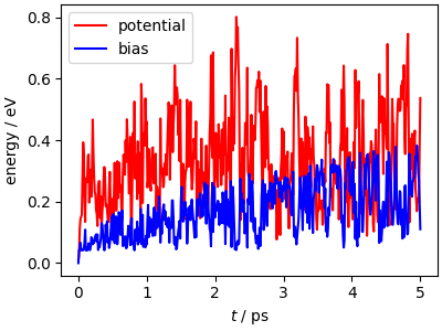
The time history of the bias is instructive, as it shows how the bias grows until the trajectory gets pushed in a new region (where the bias is zero) and then grows again. The envelope of the bias increase slows down over time, because the “well-tempered” deposition strategy reduces the height of the hills deposited in high-bias regions.

Note that the potential energy has fluctuations that are larger than the magnitude of the bias, although it shows a tendency to reach higher values as the simulation progresses. This is because only two degrees of freedom are affected by the bias, while all degrees of freedom undergo thermal fluctuations, which are dominant even for this small system.

fig, ax = plt.subplots(1, 1, figsize=(4, 3), constrained_layout=True)

ax.plot(
    2.4188843e-05 * output_data["time"],
    27.211386 * output_data["potential"],
    "r",
    label="potential",
)
ax.plot(
    2.4188843e-05 * output_data["time"],
    27.211386 * output_data["ensemble_bias"],
    "b",
    label="bias",
)

ax.set_xlabel(r"$t$ / ps")
ax.set_ylabel(r"energy / eV")
ax.legend(loc="upper left", ncols=1)
plt.show()

It’s important to keep in mind that the growing metadynamics bias can lead to deviations from the quasi-equilibrium sampling that is necessary to recover the correct properties of the rare event. It is not easy to verify this condition, but one simple diagnostics that can highlight the most evident problems is looking at the kinetic temperature of different portions of the system, computing a moving average to have a clearer signal.

def moving_average(arr, window_size):
    # Create a window of the specified size with equal weights
    window = np.ones(window_size) / window_size
    # Use the 'valid' mode to only return elements where the window fully
    # overlaps with the data
    return np.convolve(arr, window, mode="valid")


fig, ax = plt.subplots(1, 1, figsize=(4, 3), constrained_layout=True)

ax.plot(
    2.4188843e-05 * output_data["time"][50:-49],
    moving_average(output_data["temperature(O)"], 100),
    "r",
    label=r"$T_\mathrm{O}$",
)
ax.plot(
    2.4188843e-05 * output_data["time"][50:-49],
    moving_average(output_data["temperature(H)"], 100),
    "gray",
    label=r"$T_\mathrm{H}$",
)
ax.plot(
    2.4188843e-05 * output_data["time"][50:-49],
    moving_average(output_data["temperature"], 100),
    "b",
    label="T",
)

ax.set_xlabel(r"$t$ / ps")
ax.set_ylabel(r"temperature / K")
ax.legend(loc="upper left", ncols=2)
plt.show()

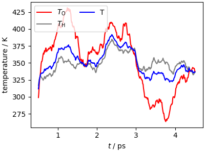
It is clear that the very high rate of biasing used in this demonstrative example leads to a temperature that is consistently higher than the target, with spikes up to 380 K and O and H atoms reaching different temperatures (i.e. equipartition is broken). While this does not affect the qualitative nature of the results, these parameters are unsuitable for a production run. NB: especially for small systems, the instantaneous kinetic temperature can deviate by a large amount from the target temperature: only the mean value has actual meaning. However, a kinetic temperature that is consistently above the target value indicates that the thermostat cannot dissipate efficiently the energy due to the growing bias.

Free energy profiles

One of the advantages of metadynamics is that it allows one to easily estimate the free-energy associated with the collective variables that are used to accelerate sampling by summing the repulsive hills that have been deposited during the run and taking the negative of the total bias at the end of the trajectory.

Even though more sophisticated strategies exist that provide explicit weighting factors to estimate the unbiased Boltzmann distribution (see e.g. Giberti et al., JCTC 2020), this simple approach is good enough for this example, and can be realized as a post-processing step using the plumed sum_hills module, that also applies a (simple) correction to the negative bias that is needed when using the well-tempered bias scaling protocol. On the command line,

plumed sum_hills --hills HILLS-md --min 0.21,-1 --max 0.31,1 --bin 100,100 \
       --outfile FES-md --stride 100 --mintozero < data/plumed-md.dat

The --stride option generates a series of files showing the estimates of \(F\) at different times along the trajectory.

with open("data/plumed-md.dat", "r") as file:
    subprocess.run(
        [
            "plumed",
            "sum_hills",
            "--hills",
            "HILLS-md",
            "--min",
            "0.21,-1",
            "--max",
            "0.31,1",
            "--bin",
            "100,100",
            "--outfile",
            "FES-md",
            "--stride",
            "100",
            "--mintozero",
        ],
        stdin=file,
        text=True,
    )

# rearrange data and converts to Å and eV
data = np.loadtxt("FES-md0.dat", comments="#")[:, :3]
xyz_0 = np.array([10, 1, 0.01036427])[:, np.newaxis, np.newaxis] * data.T.reshape(
    3, 101, 101
)
data = np.loadtxt("FES-md2.dat", comments="#")[:, :3]
xyz_2 = np.array([10, 1, 0.01036427])[:, np.newaxis, np.newaxis] * data.T.reshape(
    3, 101, 101
)
data = np.loadtxt("FES-md5.dat", comments="#")[:, :3]
xyz_5 = np.array([10, 1, 0.01036427])[:, np.newaxis, np.newaxis] * data.T.reshape(
    3, 101, 101
)

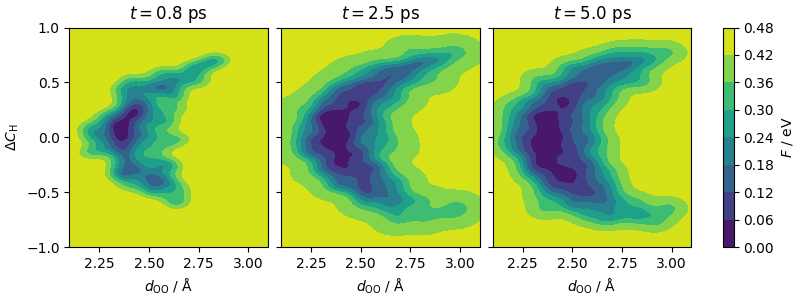
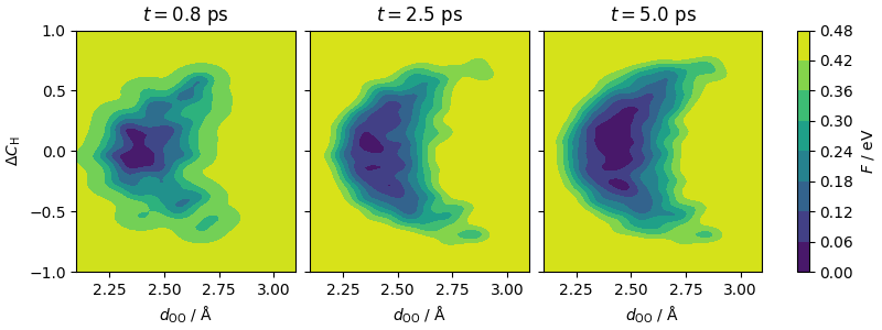
The plots show, left-to-right, the accumulation of the metadynamics bias as simulation progresses.

fig, ax = plt.subplots(
    1, 3, figsize=(8, 3), sharex=True, sharey=True, constrained_layout=True
)

cf_0 = ax[0].contourf(*xyz_0)
cf_1 = ax[1].contourf(*xyz_2)
cf_2 = ax[2].contourf(*xyz_5)
fig.colorbar(cf_2, ax=ax, orientation="vertical", label=r"$F$ / eV")
ax[0].set_ylabel(r"$\Delta C_\mathrm{H}$")
ax[0].set_xlabel(r"$d_\mathrm{OO}$ / Å")
ax[1].set_xlabel(r"$d_\mathrm{OO}$ / Å")
ax[2].set_xlabel(r"$d_\mathrm{OO}$ / Å")
ax[0].set_title(r"$t=0.8$ ps")
ax[1].set_title(r"$t=2.5$ ps")
ax[2].set_title(r"$t=5.0$ ps")
plt.show()

Biasing a path integral calculation

You can see this recipe for a brief introduction to path integral simulations with i-PI. From a practical perspective, very little needs to change with respect to the classical case.

xmlroot = ET.parse("data/input-pimd.xml").getroot()

The nbeads option determines the number of path integral replicas. The value of 8 used here is not sufficient to converge quantum statistics at 300 K (a more typical value would be around 32). There are methods to reduce the number of replicas needed for convergence, see e.g. Ceriotti and Markland, Nat. Rev. Chem. (2018) but we keep it simple here.

print(" " + ET.tostring(xmlroot.find(".//initialize"), encoding="unicode")[:23])

<initialize nbeads="8">

Centroid bias

Another detail worth discussing is that the metadynamics bias is computed exclusively on the centroid, the mean position of the ring-polymer beads. This is an extreme form of ring polymer contraction (Markland and Manolopoulos, J. Chem. Phys. (2008) that avoids computing for each replica the slowly-varying parts of the potential, but is not applied for computational savings. When performing a quantum free-energy calculation it is important to distinguish between the free-energy computed as the logarithm of the probability of observing a given configuration (that depends on the distribution of the replicas) and the free-energy taken as a tool to estimate reaction rates \(k\) in a transition-state theory fashion \(k\propto e^{-\Delta E^\ddagger/kT}\), where the energy barrier \(\Delta E^\ddagger\) is better estimated from the distribution of the centroid. See e.g. Habershon et al., Annu. Rev. Phys. Chem. (2013) for a discussion of the subtleties involved in estimating transition rates. In practice, performing this contraction step is very easy in i-PI, because for each <force> section - including that corresponding to the bias - it is possible to specify a different number of replicas. The configurations will be automatically computed by Fourier interpolation.

print("         " + ET.tostring(xmlroot.find(".//bias"), encoding="unicode"))

<bias>
  <force forcefield="plumed" nbeads="1">
    <interpolate_extras> [ doo, dc, mtd.bias ] </interpolate_extras>
  </force>
</bias>

Running the calculation

The other changes are purely cosmetic, and the calculation can be launched very easily, using several drivers to parallelize the energy evaluation over the beads (although this kind of calculations is not limited by the evaluation of the forces).

# don't rerun if the outputs already exist
ipi_process = None
if not os.path.exists("meta-pimd.out"):
    ipi_process = subprocess.Popen(["i-pi", "data/input-pimd.xml"])
    time.sleep(2)  # wait for i-PI to start
    driver_process = [
        subprocess.Popen(
            ["i-pi-driver", "-u", "-a", "zundel", "-m", "zundel"], cwd="data/"
        )
        for i in range(4)
    ]

If you run this in a notebook, you can go ahead and start loading output files _before_ i-PI has finished running by skipping this cell

# wait for simulations to finish
if ipi_process is not None:
    ipi_process.wait()
    for process in driver_process:
        process.wait()

Analysis of the simulation

A path integral simulation evolves multiple configurations at the same time, forming a ring polymer. Each replica provides a sample of the quantum mechanical configuration distribution of the atoms. To provide an overall visualization of the path integral dynamics, we load all the replicas and combine them using a utility function from the chemiscope library.`

output_data, output_desc = ipi.read_output("meta-pimd.out")
colvar_data = ipi.read_trajectory("meta-pimd.colvar_0", format="extras")[
    "doo,dc,mtd.bias"
]
pimd_traj_data = [ipi.read_trajectory(f"meta-pimd.pos_{i}.xyz") for i in range(8)]

# combines the PI beads and sets up the visualization options
traj_pimd = chemiscope.ase_merge_pi_frames(pimd_traj_data)
traj_pimd["shapes"]["paths"]["parameters"]["global"]["radius"] = 0.05
traj_pimd["properties"] = dict(
    d_OO=10 * colvar_data[:, 0],  # nm to Å
    delta_coord=colvar_data[:, 1],
    bias=27.211386 * output_data["ensemble_bias"],  # Ha to eV
    time=2.4188843e-05 * output_data["time"],
)
traj_pimd["settings"] = chemiscope.quick_settings(
    x="d_OO",
    y="delta_coord",
    z="bias",
    color="time",
    trajectory=True,
    structure_settings=dict(
        bonds=False,
        atoms=False,
        keepOrientation=True,
        unitCell=False,
        shape=[
            "paths",
        ],
    ),
)
traj_pimd["settings"]["target"] = "structure"

Visualize the trajectory. Note the similar behavior as for the classical trajectory, and the delocalization of the protons

chemiscope.show(**traj_pimd)

×

Free energy plots

The free energy profiles relative to \(\Delta C_\mathrm{H}\) and \(d_\mathrm{OO}\) can be computed exactly as for the classical trajectory, using the sum_hills module.

with open("data/plumed-pimd.dat", "r") as file:
    subprocess.run(
        [
            "plumed",
            "sum_hills",
            "--hills",
            "HILLS-pimd",
            "--min",
            "0.21,-1",
            "--max",
            "0.31,1",
            "--bin",
            "100,100",
            "--outfile",
            "FES-pimd",
            "--stride",
            "100",
            "--mintozero",
        ],
        stdin=file,
        text=True,
    )

# rearrange data and converts to Å and eV
data = np.loadtxt("FES-pimd0.dat", comments="#")[:, :3]
xyz_pi_0 = np.array([10, 1, 0.01036427])[:, np.newaxis, np.newaxis] * data.T.reshape(
    3, 101, 101
)
data = np.loadtxt("FES-pimd2.dat", comments="#")[:, :3]
xyz_pi_2 = np.array([10, 1, 0.01036427])[:, np.newaxis, np.newaxis] * data.T.reshape(
    3, 101, 101
)
data = np.loadtxt("FES-pimd5.dat", comments="#")[:, :3]
xyz_pi_5 = np.array([10, 1, 0.01036427])[:, np.newaxis, np.newaxis] * data.T.reshape(
    3, 101, 101
)

Just as for a classical run, the metadynamics bias progressively pushes the centroid (and the beads that are distributed around it) to sample a wider portion of the collective-variable space.

fig, ax = plt.subplots(
    1, 3, figsize=(8, 3), sharex=True, sharey=True, constrained_layout=True
)

cf_0 = ax[0].contourf(*xyz_pi_0)
cf_1 = ax[1].contourf(*xyz_pi_2)
cf_2 = ax[2].contourf(*xyz_pi_5)
fig.colorbar(cf_2, ax=ax, orientation="vertical", label=r"$F$ / eV")
ax[0].set_ylabel(r"$\Delta C_\mathrm{H}$")
ax[0].set_xlabel(r"$d_\mathrm{OO}$ / Å")
ax[1].set_xlabel(r"$d_\mathrm{OO}$ / Å")
ax[2].set_xlabel(r"$d_\mathrm{OO}$ / Å")
ax[0].set_title(r"$t=0.8$ ps")
ax[1].set_title(r"$t=2.5$ ps")
ax[2].set_title(r"$t=5.0$ ps")
plt.show()

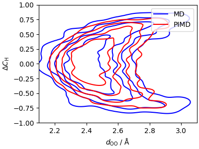
Assessing quantum nuclear effects

The effect of nuclear quantization on the centroid free-energy is relatively small, despite the large delocalization of the protons in the PIMD calculation. Looking more carefully at the two distributions, one can notice that in the high-\(d_\mathrm{OO}\) region there is higher delocalisation of the proton.

fig, ax = plt.subplots(
    1, 1, figsize=(4, 3), sharex=True, sharey=True, constrained_layout=True
)

levels = np.linspace(0, 0.5, 6)
cp1 = ax.contour(*xyz_5, colors="b", levels=levels)
cp2 = ax.contour(*xyz_pi_5, colors="r", levels=levels)
ax.set_ylabel(r"$\Delta C_\mathrm{H}$")
ax.set_xlabel(r"$d_\mathrm{OO}$ / Å")
ax.legend(
    handles=[
        plt.Line2D([0], [0], color="b", label="MD"),
        plt.Line2D([0], [0], color="r", label="PIMD"),
    ]
)
plt.show()

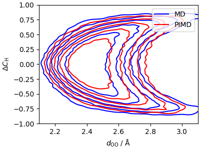
To get a clear signal, we need better-converged calculations; the data/ folder contains inputs for these “high quality” runs, and free-energies obtained from them. The results confirm the lowering of the free-energy barrier for the \(\mathrm{H_3O^+ + H_2O} \rightarrow \mathrm{H_2O + H_3O^+}\) transition.

with bz2.open("data/FES-md_hiq.bz2", "rt") as f:
    data = np.loadtxt(f, comments="#")[:, :3]
xyz_md_hiq = np.array([10, 1, 0.01036427])[:, np.newaxis, np.newaxis] * data.T.reshape(
    3, 101, 101
)
with bz2.open("data/FES-pimd_hiq.bz2", "rt") as f:
    data = np.loadtxt(f, comments="#")[:, :3]
xyz_pi_hiq = np.array([10, 1, 0.01036427])[:, np.newaxis, np.newaxis] * data.T.reshape(
    3, 101, 101
)

fig, ax = plt.subplots(
    1, 1, figsize=(4, 3), sharex=True, sharey=True, constrained_layout=True
)

levels = np.linspace(0, 0.5, 6)
cp1 = ax.contour(*xyz_md_hiq, colors="b", levels=levels)
cp2 = ax.contour(*xyz_pi_hiq, colors="r", levels=levels)
ax.set_ylabel(r"$\Delta C_\mathrm{H}$")
ax.set_xlabel(r"$d_\mathrm{OO}$ / Å")
ax.legend(
    handles=[
        plt.Line2D([0], [0], color="b", label="MD"),
        plt.Line2D([0], [0], color="r", label="PIMD"),
    ]
)
plt.show()

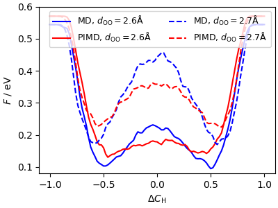
The lowering of the barrier for proton hopping is clearly seen by taking 1D slices of the free energy at different O-O separations.

fig, ax = plt.subplots(
    1, 1, figsize=(4, 3), sharex=True, sharey=True, constrained_layout=True
)

ax.plot(
    xyz_md_hiq[1, :, 50], xyz_md_hiq[2, :, 50], "b", label=r"MD, $d_\mathrm{OO}=2.6 $Å"
)
ax.plot(
    xyz_pi_hiq[1, :, 50],
    xyz_pi_hiq[2, :, 50],
    "r",
    label=r"PIMD, $d_\mathrm{OO}=2.6 $Å",
)
ax.plot(
    xyz_md_hiq[1, :, 60],
    xyz_md_hiq[2, :, 60],
    "b--",
    label=r"MD, $d_\mathrm{OO}=2.7 $Å",
)
ax.plot(
    xyz_pi_hiq[1, :, 60],
    xyz_pi_hiq[2, :, 60],
    "r--",
    label=r"PIMD, $d_\mathrm{OO}=2.7 $Å",
)
ax.set_ylim(0.08, 0.6)
ax.legend(ncols=2, loc="upper right", fontsize=9)
ax.set_ylabel(r"$F$ / eV")
ax.set_xlabel(r"$\Delta C_\mathrm{H}$")
plt.show()

This model system is representative of the behavior of protons along a hydrogen bond in different conditions, where the environment determines the typical O-O separation, and whether the proton is shared (as in high pressure ice X) or preferentially attached to one of the two molecules. Zero-point energy (and to a lesser extent tunneling) increases the delocalization, and reduces the barrier for an excess proton to hop between water molecues.