LODE Tutorial

Authors:

Philip Loche @PicoCentauri, Kevin Huguenin-Dumittan @kvhuguenin

This tutorial explains how Long range equivariant descriptors can be constructed using rascaline and the resulting descriptors be used to construct a linear model with equisolve

First, import all the necessary packages

import ase.io
import matplotlib.pyplot as plt
import metatensor
import numpy as np
from equisolve.numpy.models.linear_model import Ridge
from equisolve.utils.convert import ase_to_tensormap
from rascaline import AtomicComposition, LodeSphericalExpansion, SphericalExpansion
from rascaline.utils import PowerSpectrum

Step 0: Prepare Data Set

Get structures

We take a small subset of the dimer dataset from A. Grisafi et al., 2021 for which we additionally calculated the forces. Each structure in the dataset contains two small organic molecules which are extended along a certain direction in the subsequent structures.

For speeding up the calculations we already selected the first 130 structures of the charge-charge molecule pairs.

frames = ase.io.read("charge-charge.xyz", ":")

Convert target properties to metatensor format

If we want to train models using the equisolve package, we need to convert the target properties (in this case, the energies and forces) into the appropriate format #justequistorethings

y = ase_to_tensormap(frames, energy="energy", forces="forces")

Step 1: Compute short-range and LODE features

Define hypers and get the expansion coefficients \(\langle anlm | \rho_i \rangle\) and \(\langle anlm | V_i \rangle\)

The short-range and long-range descriptors have very similar hyperparameters. We highlight the differences below.

We first define the hyperparameters for the short-range (SR) part. These will be used to create SOAP features.

SR_HYPERS = {
    "cutoff": 3.0,
    "max_radial": 6,
    "max_angular": 2,
    "atomic_gaussian_width": 0.3,
    "center_atom_weight": 1.0,
    "radial_basis": {"Gto": {}},
    "cutoff_function": {"ShiftedCosine": {"width": 0.5}},
}

And next the hyperparaters for the LODE / long-range (LR) part

LR_HYPERS = {
    # Cutoff on which to project potential density
    "cutoff": 3.0,
    # keep max_radial slightly smaller than for SR part
    "max_radial": 3,
    # max_angular should be <= 4, more precisely, max_angular + potential_exponent < 10
    "max_angular": 2,
    # keep at >=1, WARNING: CUBIC SCALING, do not use values <0.5
    "atomic_gaussian_width": 3.0,
    "center_atom_weight": 1.0,
    "radial_basis": {"Gto": {}},
    # the exponent p that determines the 1/r^p potential
    "potential_exponent": 1,
}

We then use the above defined hyperparaters to define the per atom short range (sr) and long range (sr) descriptors.

calculator_sr = SphericalExpansion(**SR_HYPERS)
calculator_lr = LodeSphericalExpansion(**LR_HYPERS)

Note that LODE requires periodic systems. Therefore, if the data set does not come with periodic boundary conditions by default you can not use the data set and you will face an error if you try to compute the features.

As you notices the calculation of the long range features takes significant more time compared to the sr features.

Taking a look at the output we find that the resulting metatensor.TensorMap are quite similar in their structure. The short range metatensor.TensorMap contains more blocks due to the higher max_angular paramater we choosed above.

Generate the rotational invariants (power spectra)

Rotationally invariant features can be obtained by taking two of the calculators that were defines above.

For the short-range part, we use the SOAP vector which is obtained by computing the invariant combinations of the form \(\rho \otimes \rho\).

ps_calculator_sr = PowerSpectrum(calculator_sr, calculator_sr)
ps_sr = ps_calculator_sr.compute(frames, gradients=["positions"])

We calculate gradients with respect to pistions by providing the gradients=["positions"] option to the rascaline.calculators.CalculatorBase.compute() method.

For the long-range part, we combine the long-range descriptor \(V\) with one a short-range density \(\rho\) to get \(\rho \otimes V\) features.

ps_calculator_lr = PowerSpectrum(calculator_sr, calculator_lr)
ps_lr = ps_calculator_lr.compute(systems=frames, gradients=["positions"])

Step 2: Building a Simple Linear SR + LR Model with energy baselining

Preprocessing (model dependent)

For our current model, we do not wish to treat the individual center and neighbor species separately. Thus, we move the "species_center" key into the sample direction, over which we will later sum over.

ps_sr = ps_sr.keys_to_samples("species_center")
ps_lr = ps_lr.keys_to_samples("species_center")

For linear models only: Sum features up over atoms (samples) in the same structure.

sample_names_to_sum = ["center", "species_center"]

ps_sr = metatensor.sum_over_samples(ps_sr, sample_names=sample_names_to_sum)
ps_lr = metatensor.sum_over_samples(ps_lr, sample_names=sample_names_to_sum)

Initialize tensormaps for energy baselining

We add a simple extra descriptor rascaline.AtomicComposition that stores how many atoms of each chemical species are contained in the structures. This is used for energy baselining.

calculator_co = AtomicComposition(per_structure=False)
descriptor_co = calculator_co.compute(frames, gradients=["positions"])

co = descriptor_co.keys_to_properties(["species_center"])
co = metatensor.sum_over_samples(co, sample_names=["center"])

The rascaline.AtomicComposition calculator also allows to directly perform the the sum over center atoms by using the following lines.

descriptor_co = AtomicComposition(per_structure=True).compute(**compute_args)
co = descriptor_co.keys_to_properties(["species_center"])

Stack all the features together for linear model

A linear model on SR + LR features can be thought of as a linear model built on a feature vector that is simply the concatenation of the SR and LR features.

Furthermore, energy baselining can be performed by concatenating the information about chemical species as well. There is an metatensor function called metatensor.join() for this purpose. Formally, we can write for the SR model.

X_sr: \(1 \oplus \left(\rho \otimes \rho\right)\)

X_sr = metatensor.join([co, ps_sr], axis="properties")

We used the axis="properties" parameter since we want to concatenate along the features/properties dimensions.

For the long range model we can formerly write

X_lr: \(1 \oplus \left(\rho \otimes \rho\right) \oplus \left(\rho \otimes V\right)\)

X_lr = metatensor.join([co, ps_sr, ps_lr], axis="properties")

The features are now ready! Let us now perform some actual learning. Below we initialize two instances of the equisolve.numpy.models.linear_model.Ridge class. equisolve.numpy.models.linear_model.Ridge will perform a regression with respect to "values" (energies) and "positions" gradients (forces).

If you only want a fit with respect to energies you can remove the gradients with metatensor.remove_gradients()

clf_sr = Ridge()
clf_lr = Ridge()

Split training and target data into train and test dat

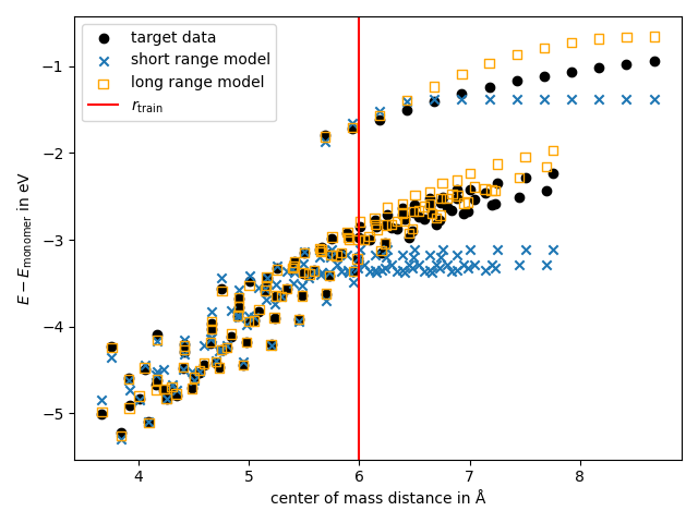
Split the training and the test data by the distance \(r_{\rm train}=6\,\mathrm{Å}\) between the center of mass of the two molecules. A structure with a \(r_{\rm train}<6 {\rm Å}\) is used for training.

r_cut = 6.0

We calculate the indices from the dataset by list comprehension. The center of mass distance is stored in the "distance"" attribute.

idx_train = [i for i, f in enumerate(frames) if f.info["distance"] < r_cut]
idx_test = [i for i, f in enumerate(frames) if f.info["distance"] >= r_cut]

For doing the split we define two Labels instances and combine them in a List.

samples_train = metatensor.Labels(["structure"], np.reshape(idx_train, (-1, 1)))
samples_test = metatensor.Labels(["structure"], np.reshape(idx_test, (-1, 1)))
grouped_labels = [samples_train, samples_test]

That we use as input to the metatensor.split() function

X_sr_train, X_sr_test = metatensor.split(
    X_sr, axis="samples", grouped_labels=grouped_labels
)

X_lr_train, X_lr_test = metatensor.split(
    X_lr, axis="samples", grouped_labels=grouped_labels
)

y_train, y_test = metatensor.split(y, axis="samples", grouped_labels=grouped_labels)

Fit the model

For this model, we use a very simple regularization scheme where all features are regularized in the same way (the amount being controlled by the parameter alpha). For more advanced regularization schemes (regularizing energies and forces differently and/or the SR and LR parts differently), see further down.

clf_sr.fit(X_sr_train, y_train, alpha=1e-6)
clf_lr.fit(X_lr_train, y_train, alpha=1e-6)

<equisolve.numpy.models.linear_model.NumpyRidge object at 0x7fdb3d3d8210>

Evaluation

For evaluating the model we calculate the RMSEs using the score() method. With the parameter_key parameter we select which RMSE should be calculated.

print(
    "SR: RMSE energies = "
    f"{clf_sr.score(X_sr_test, y_test, parameter_key='values')[0]:.3f} eV"
)
print(
    "SR: RMSE forces = "
    f"{clf_sr.score(X_sr_test, y_test, parameter_key='positions')[0]:.3f} eV/Å"
)

print(
    "LR: RMSE energies = "
    f"{clf_lr.score(X_lr_test, y_test, parameter_key='values')[0]:.3f} eV"
)
print(
    "LR: RMSE forces = "
    f"{clf_lr.score(X_lr_test, y_test, parameter_key='positions')[0]:.3f} eV/Å"
)

SR: RMSE energies = 0.557 eV
SR: RMSE forces = 0.188 eV/Å
LR: RMSE energies = 0.158 eV
LR: RMSE forces = 0.178 eV/Å

We find that the RMSE of the energy and the force of the LR model is smaller compared to the SR model. From this we conclude that the LR model performs better for the selection of the dataset.

We additionally, can plot of the binding energy as a function of the distance. For the plot we select some properties from the dataset

dist = np.array([f.info["distance"] for f in frames])
energies = np.array([f.info["energy"] for f in frames])
monomer_energies = np.array([f.info["energyA"] + f.info["energyB"] for f in frames])

and select only the indices corresponding to our test set.

Next we calculate the predicted SR and LR TensorMaps.

y_sr_pred = clf_sr.predict(X_sr)
y_lr_pred = clf_lr.predict(X_lr)

And, finally perform the plot.

plt.scatter(
    dist, y.block().values[:, 0] - monomer_energies, label="target data", color="black"
)

plt.scatter(
    dist,
    y_sr_pred.block().values[:, 0] - monomer_energies,
    label="short range model",
    marker="x",
)

plt.scatter(
    dist,
    y_lr_pred.block().values[:, 0] - monomer_energies,
    label="long range model",
    marker="s",
    facecolor="None",
    edgecolor="orange",
)

plt.xlabel("center of mass distance in Å")
plt.ylabel(r"$E - E_\mathrm{monomer}$ in eV")
plt.axvline(r_cut, c="red", label=r"$r_\mathrm{train}$")

plt.legend()
plt.tight_layout()
plt.show()