Generalized Convex Hull construction for the polymorphs of ROY

Authors:

Michele Ceriotti @ceriottm

This notebook analyzes the structures of 264 polymorphs of ROY, from Beran et Al, Chemical Science (2022), comparing the conventional density-energy convex hull with a Generalized Convex Hull (GCH) analysis (see Anelli et al., Phys. Rev. Materials (2018)). It uses features computed with rascaline and uses the directional convex hull function from scikit-matter to make the figure.

The GCH construction aims at determining structures, among a collection of candidate configurations, that are stable or have the potential of being stabilized by appropriate thermodynamic boundary conditions (pressure, doping, external fields, …). It does so by using microscopic descriptors to determine the diversity of structures, and assumes that configurations that are stable relative to other configurations with similar descriptors are those that could be made “locally” stable by suitable synthesis conditions.

# sphinx_gallery_thumbnail_number = 3
import chemiscope
import matplotlib.tri
import numpy as np
from matplotlib import pyplot as plt
from metatensor import mean_over_samples
from rascaline import SoapPowerSpectrum
from sklearn.decomposition import PCA
from skmatter.datasets import load_roy_dataset
from skmatter.sample_selection import DirectionalConvexHull

Loads the structures (that also contain properties in the info field)

roy_data = load_roy_dataset()

structures = roy_data["structures"]

density = np.array([s.info["density"] for s in structures])
energy = np.array([s.info["energy"] for s in structures])
structype = np.array([s.info["type"] for s in structures])
iknown = np.where(structype == "known")[0]
iothers = np.where(structype != "known")[0]

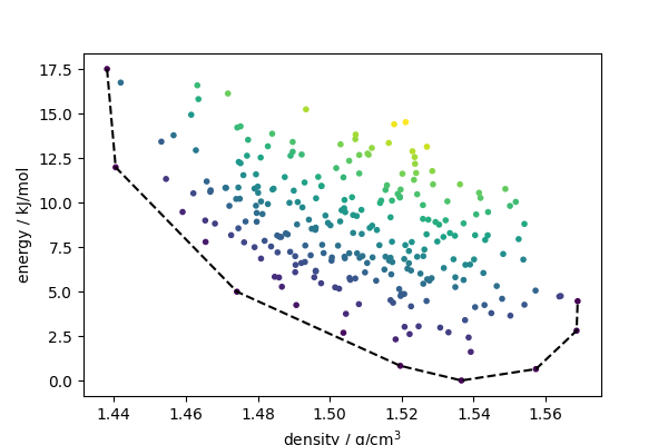
Energy-density hull

The Directional Convex Hull routines can be used to compute a conventional density-energy hull (see Hautier (2014) for a pedagogic introduction to the convex hull construction in the context of atomistic simulations).

dch_builder = DirectionalConvexHull(low_dim_idx=[0])
dch_builder.fit(density.reshape(-1, 1), energy)

<skmatter.sample_selection._base.DirectionalConvexHull object at 0x7fd930a56a10>

We can get the indices of the selection, and compute the distance from the hull

sel = dch_builder.selected_idx_
dch_dist = dch_builder.score_samples(density.reshape(-1, 1), energy)

Hull energies

Structures on the hull are stable with respect to synthesis at constant molar volume. Any other structure would lower the energy by decomposing into a mixture of the two nearest structures along the hull. Given that the lattice energy is an imperfect proxy for the free energy, and that synthesis can be performed in other ways than by fixing the density, structures that are not exactly on the hull might also be stable. One can compute a “hull energy” as an indication of how close these structures are to being stable.

fig, ax = plt.subplots(1, 1, figsize=(6, 4))
ax.scatter(density, energy, c=dch_dist, marker=".")
ssel = sel[np.argsort(density[sel])]
ax.plot(density[ssel], energy[ssel], "k--")
ax.set_xlabel("density / g/cm$^3$")
ax.set_ylabel("energy / kJ/mol")
plt.show()

print(
    f"Mean hull energy for 'known' stable structures {dch_dist[iknown].mean()} kJ/mol"
)
print(f"Mean hull energy for 'other' structures {dch_dist[iothers].mean()} kJ/mol")

Mean hull energy for 'known' stable structures 1.816657381014075 kJ/mol
Mean hull energy for 'other' structures 6.312730486304906 kJ/mol

Interactive visualization

You can also visualize the hull with chemiscope in a juptyer notebook.

cs = chemiscope.show(
    structures,
    dict(
        energy=energy,
        density=density,
        hull_energy=dch_dist,
        structure_type=structype,
    ),
    settings={
        "map": {
            "x": {"property": "density"},
            "y": {"property": "energy"},
            "color": {"property": "hull_energy"},
            "symbol": "structure_type",
            "size": {"factor": 35},
        },
        "structure": [{"unitCell": True, "supercell": {"0": 2, "1": 2, "2": 2}}],
    },
)
cs

×

Save chemiscope file in a format that can be shared and viewed on chemiscope.org

cs.save("roy_ch.json.gz")

Generalized Convex Hull

A GCH is a similar construction, in which generic structural descriptors are used in lieu of composition, density or other thermodynamic constraints. The idea is that configurations that are found close to the GCH are locally stable with respect to structurally-similar configurations. In other terms, one can hope to find a thermodynamic constraint (i.e. synthesis conditions) that act differently on these structures in comparison with the others, and may potentially stabilize them.

Compute structural descriptors

A first step is to computes suitable ML descriptors. Here we have used rascaline to evaluate average SOAP features for the structures. If you don’t want to install these dependencies for this example you can also use the pre-computed features, but you can use this as a stub to apply this analysis to other chemical systems

hypers = {
    "cutoff": 4,
    "max_radial": 6,
    "max_angular": 4,
    "atomic_gaussian_width": 0.7,
    "cutoff_function": {"ShiftedCosine": {"width": 0.5}},
    "radial_basis": {"Gto": {"accuracy": 1e-6}},
    "center_atom_weight": 1.0,
}
calculator = SoapPowerSpectrum(**hypers)
rho2i = calculator.compute(structures)
rho2i = rho2i.keys_to_samples(["species_center"]).keys_to_properties(
    ["species_neighbor_1", "species_neighbor_2"]
)
rho2i_structure = mean_over_samples(rho2i, sample_names=["center", "species_center"])
np.savez("roy_features.npz", feats=rho2i_structure.block(0).values)


# features = roy_data["features"]
features = rho2i_structure.block(0).values

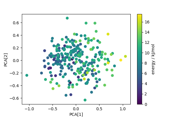
PCA projection

Computes PCA projection to generate low-dimensional descriptors that reflect structural diversity. Any other dimensionality reduction scheme could be used in a similar fashion.

pca = PCA(n_components=4)
pca_features = pca.fit_transform(features)

fig, ax = plt.subplots(1, 1, figsize=(6, 4))
scatter = ax.scatter(pca_features[:, 0], pca_features[:, 1], c=energy)
ax.set_xlabel("PCA[1]")
ax.set_ylabel("PCA[2]")
cbar = fig.colorbar(scatter, ax=ax)
cbar.set_label("energy / kJ/mol")
plt.show()

Builds the Generalized Convex Hull

Builds a convex hull on the first two PCA features

dch_builder = DirectionalConvexHull(low_dim_idx=[0, 1])
dch_builder.fit(pca_features, energy)
sel = dch_builder.selected_idx_
dch_dist = dch_builder.score_samples(pca_features, energy)

Generates a 3D Plot

triang = matplotlib.tri.Triangulation(pca_features[sel, 0], pca_features[sel, 1])
fig = plt.figure(figsize=(7, 5), tight_layout=True)
ax = fig.add_subplot(projection="3d")
ax.plot_trisurf(triang, energy[sel], color="gray")
ax.scatter(pca_features[:, 0], pca_features[:, 1], energy, c=dch_dist)
ax.set_xlabel("PCA[1]")
ax.set_ylabel("PCA[2]")
ax.set_zlabel("energy / kJ/mol\n \n", labelpad=11)
ax.view_init(25, 110)
plt.show()

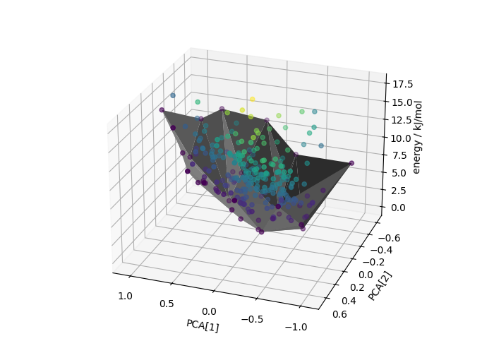
The GCH construction improves the separation between the hull energies of “known” and hypothetical polymorphs (compare with the density-energy values above)

print(
    f"Mean hull energy for 'known' stable structures {dch_dist[iknown].mean()} kJ/mol"
)
print(f"Mean hull energy for 'other' structures {dch_dist[iothers].mean()} kJ/mol")

Mean hull energy for 'known' stable structures 0.8537845044709435 kJ/mol
Mean hull energy for 'other' structures 5.1988715818497795 kJ/mol

Visualize in a chemiscope widget

for i, f in enumerate(structures):
    for j in range(len(pca_features[i])):
        f.info["pca_" + str(j + 1)] = pca_features[i, j]
structure_properties = chemiscope.extract_properties(structures)
structure_properties.update({"per_atom_energy": energy, "hull_energy": dch_dist})

# You can save a chemiscope file to disk (for viewing on chemiscope.org)

chemiscope.write_input(
    "roy_gch.json.gz",
    frames=structures,
    properties=structure_properties,
    meta={
        "name": "GCH for ROY polymorphs",
        "description": """
Demonstration of the Generalized Convex Hull construction for
polymorphs of the ROY molecule. Molecules that are closest to
the hull built on PCA-based structural descriptors and having the
internal energy predicted by electronic-structure calculations as
the z axis are the most thermodynamically stable. Indeed most of the
known polymorphs of ROY are on (or very close) to this hull.
""",
        "authors": ["Michele Ceriotti <[email protected]>"],
        "references": [
            'A. Anelli, E. A. Engel, C. J. Pickard, and M. Ceriotti, \
            "Generalized convex hull construction for materials discovery," \
            Physical Review Materials 2(10), 103804 (2018).',
            'G. J. O. Beran, I. J. Sugden, C. Greenwell, D. H. Bowskill, \
            C. C. Pantelides, and C. S. Adjiman, "How many more polymorphs of \
            ROY remain undiscovered," Chem. Sci. 13(5), 1288–1297 (2022).',
        ],
    },
    settings={
        "map": {
            "x": {"property": "pca_1"},
            "y": {"property": "pca_2"},
            "z": {"property": "energy"},
            "symbol": "type",
            "color": {"property": "hull_energy"},
            "size": {
                "factor": 35,
                "mode": "linear",
                "property": "",
                "reverse": True,
            },
        },
        "structure": [
            {
                "bonds": True,
                "unitCell": True,
                "keepOrientation": True,
            }
        ],
    },
)

… and also load one as an interactive viewer

chemiscope.show_input("roy_gch.json.gz")

×