Note
Go to the end to download the full example code.
A ML model for the electron density of states
- Authors:
How Wei Bin @HowWeiBin
This tutorial would go through the entire machine learning framework for the electronic density of states (DOS). It will cover the construction of the DOS and SOAP descriptors from ase Atoms and eigenenergy results. A simple neural network will then be constructed and the model parameters, along with the energy reference will be optimized during training. A total of three energy reference will be used, the average Hartree potential, the Fermi level, and an optimized energy reference starting from the Fermi level energy reference. The performance of each model is then compared.
First, lets begin by importing the necessary packages and helper functions
import os
import zipfile

import ase
import ase.io
import matplotlib.pyplot as plt
import numpy as np
import requests
import torch
from featomic import SoapPowerSpectrum
from scipy.interpolate import CubicHermiteSpline, interp1d
from scipy.optimize import brentq
from torch.utils.data import BatchSampler, DataLoader, Dataset, RandomSampler
Step 0: Load Structures and Eigenenergies
Downloading and Extracting Data
Loading Data
Find range of eigenenergies
We take a small subset of 104 structures in the Si dataset from Bartok et al., 2018 <https://journals.aps.org/prx/abstract/10.1103/PhysRevX.8.041048>. Each structure in the dataset contains two atoms.
1) Downloading and Extracting Data
filename = "dataset.zip"
if not os.path.exists(filename):
    url = "https://github.com/HowWeiBin/datasets/archive/refs/tags/Silicon-Diamonds.zip"
    response = requests.get(url)
    response.raise_for_status()
    with open(filename, "wb") as f:
        f.write(response.content)

with zipfile.ZipFile("./dataset.zip", "r") as zip_ref:
    zip_ref.extractall("./")
2) Loading Data
structures = ase.io.read("./datasets-Silicon-Diamonds/diamonds.xyz", ":")
n_structures = len(structures)
n_atoms = torch.tensor([len(i) for i in structures])
eigenenergies = torch.load("./datasets-Silicon-Diamonds/diamond_energies.pt")
k_normalization = torch.tensor(
    [len(i) for i in eigenenergies]
)  # Calculates number of kpoints sampled per structure
print(f"Total number of structures: {len(structures)}")
Total number of structures: 104
3) Find range of eigenenergies
# Process eigenenergies to flattened torch tensors

total_eigenenergies = [torch.flatten(torch.tensor(i)) for i in eigenenergies]

# Get lowest and highest value of eigenenergies to know the range of eigenenergies

all_eigenenergies = torch.hstack(total_eigenenergies)
minE = torch.min(all_eigenenergies)
maxE = torch.max(all_eigenenergies)
print(f"The lowest eigenenergy in the dataset is {minE:.3}")
print(f"The highest eigenenergy in the dataset is {maxE:.3}")
The lowest eigenenergy in the dataset is -20.5
The highest eigenenergy in the dataset is 8.65
Step 1: Constructing the DOS with different energy references
Construct the DOS using the original reference
Calculate the Fermi level from the DOS
Build a set of eigenenergies, with the energy reference set to the fermi level
Truncate the DOS energy window so that the DOS is well-defined at each point
Construct the DOS in the truncated energy window under both references
Construct Splines for the DOS to facilitate interpolation during model training
1) Construct the DOS using the original reference
The DOS will first be constructed from the full set of eigenenergies to determine the Fermi level of each structure. The original reference is the Average Hartree Potential in this example.
# To ensure that all the eigenenergies are fully represented after
# gaussian broadening, the energy axis of the DOS extends
# 3eV wider than the range of values for the eigenenergies
energy_lower_bound = minE - 1.5
energy_upper_bound = maxE + 1.5

# Gaussian Smearing for the eDOS, 0.3eV is the appropriate value for this dataset

sigma = torch.tensor(0.3)
energy_interval = 0.05
# energy axis, with a grid interval of 0.05 eV

x_dos = torch.arange(energy_lower_bound, energy_upper_bound, energy_interval)
print(
    f"The energy axis ranges from {energy_lower_bound:.3} to \
{energy_upper_bound:.3}, consisting of {len(x_dos)} grid points"
)

# normalization factor for each DOS, factor of 2 is included
# because each eigenenergy can be occupied by 2 electrons

normalization = 2 * (
    1 / torch.sqrt(2 * torch.tensor(np.pi) * sigma**2) / n_atoms / k_normalization
)

total_edos = []

for structure_eigenenergies in total_eigenenergies:
    e_dos = torch.sum(
        # Builds a gaussian on each eigenenergy
        # and calculates the value on each grid point
        torch.exp(-0.5 * ((x_dos - structure_eigenenergies.view(-1, 1)) / sigma) ** 2),
        dim=0,
    )
    total_edos.append(e_dos)

total_edos = torch.vstack(total_edos)
total_edos = (total_edos.T * normalization).T

print(f"The final shape of all the DOS in the dataset is: {list(total_edos.shape)}")
The energy axis ranges from -22.0 to 10.1, consisting of 644 grid points
The final shape of all the DOS in the dataset is: [104, 644]
2) Calculate the Fermi level from the DOS
Now we integration the DOS, and then use cubic interpolation and brentq to calculate the fermi level. Since only the 4 valence electrons in Silicon are represented in this energy range, we take the point where the DOS integrates to 4 as the fermi level.
fermi_levels = []
total_i_edos = torch.cumulative_trapezoid(
    total_edos, x_dos, axis=1
)  # Integrate the DOS along the energy axis
for i in total_i_edos:
    interpolated = interp1d(
        x_dos[:-1], i - 4, kind="cubic", copy=True, assume_sorted=True
    )  # We use i-4 because Silicon has 4 electrons in this energy range
    Ef = brentq(
        interpolated, x_dos[0] + 0.1, x_dos[-1] - 0.1
    )  # Fermi Level is the point where the (integrated DOS - 4) = 0
    # 0.1 is added and subtracted to prevent brentq from going out of range
    fermi_levels.append(Ef)
fermi_levels = torch.tensor(fermi_levels)
3) Build a set of eigenenergies, with the energy reference set to the fermi level
Using the fermi levels, we are now able to change the energy reference of the eigenenergies to the fermi level
total_eigenenergies_Ef = []
for index, energies in enumerate(total_eigenenergies):
    total_eigenenergies_Ef.append(energies - fermi_levels[index])

all_eigenenergies_Ef = torch.hstack(total_eigenenergies_Ef)

minE_Ef = torch.min(all_eigenenergies_Ef)
maxE_Ef = torch.max(all_eigenenergies_Ef)
print(f"The lowest eigenenergy using the fermi level energy reference is {minE_Ef:.3}")
print(f"The highest eigenenergy using the fermi level energy reference is {maxE_Ef:.3}")
The lowest eigenenergy using the fermi level energy reference is -13.8
The highest eigenenergy using the fermi level energy reference is 14.9
4) Truncate the DOS energy window so that the DOS is well-defined at each point
With the fermi levels, we can also truncate the energy window for DOS prediction. In this example, we truncate the energy window such that it is 3eV above the highest Fermi level in the dataset.
# For the Average Hartree Potential energy reference
x_dos_H = torch.arange(minE - 1.5, max(fermi_levels) + 3, energy_interval)

# For the Fermi Level Energy Reference, all the Fermi levels in the dataset is 0eV
x_dos_Ef = torch.arange(minE_Ef - 1.5, 3, energy_interval)
5) Construct the DOS in the truncated energy window under both references
Here we construct 2 different targets where they differ in the energy reference chosen. These targets will then be treated as different datasets for the model to learn on.
# For the Average Hartree Potential energy reference

total_edos_H = []

for structure_eigenenergies_H in total_eigenenergies:
    e_dos = torch.sum(
        torch.exp(
            -0.5 * ((x_dos_H - structure_eigenenergies_H.view(-1, 1)) / sigma) ** 2
        ),
        dim=0,
    )
    total_edos_H.append(e_dos)

total_edos_H = torch.vstack(total_edos_H)
total_edos_H = (total_edos_H.T * normalization).T


# For the Fermi Level Energy Reference

total_edos_Ef = []

for structure_eigenenergies_Ef in total_eigenenergies_Ef:
    e_dos = torch.sum(
        torch.exp(
            -0.5 * ((x_dos_Ef - structure_eigenenergies_Ef.view(-1, 1)) / sigma) ** 2
        ),
        dim=0,
    )
    total_edos_Ef.append(e_dos)

total_edos_Ef = torch.vstack(total_edos_Ef)
total_edos_Ef = (total_edos_Ef.T * normalization).T
6) Construct Splines for the DOS to facilitate interpolation during model training
Building Cubic Hermite Splines on the DOS on the truncated energy window to facilitate interpolation during training. Cubic Hermite Splines takes in information on the value and derivative of a function at a point to build splines. Thus, we will have to compute both the value and derivative at each spline position
# Functions to compute the value and derivative of the DOS at each energy value, x
def edos_value(x, eigenenergies, normalization):
    e_dos_E = (
        torch.sum(
            torch.exp(-0.5 * ((x - eigenenergies.view(-1, 1)) / sigma) ** 2), dim=0
        )
        * normalization
    )

    return e_dos_E


def edos_derivative(x, eigenenergies, normalization):
    dfn_dos_E = (
        torch.sum(
            torch.exp(-0.5 * ((x - eigenenergies.view(-1, 1)) / sigma) ** 2)
            * (-1 * ((x - eigenenergies.view(-1, 1)) / sigma) ** 2),
            dim=0,
        )
        * normalization
    )

    return dfn_dos_E


total_splines_H = []
# the splines have a higher energy range in case the shift is high
spline_positions_H = torch.arange(minE - 2, max(fermi_levels) + 6, energy_interval)

for index, structure_eigenenergies_H in enumerate(total_eigenenergies):
    e_dos_H = edos_value(
        spline_positions_H, structure_eigenenergies_H, normalization[index]
    )
    e_dos_H_grad = edos_derivative(
        spline_positions_H, structure_eigenenergies_H, normalization[index]
    )
    spliner = CubicHermiteSpline(spline_positions_H, e_dos_H, e_dos_H_grad)
    total_splines_H.append(torch.tensor(spliner.c))

total_splines_H = torch.stack(total_splines_H)

total_splines_Ef = []
spline_positions_Ef = torch.arange(minE_Ef - 2, 6, energy_interval)

for index, structure_eigenenergies_Ef in enumerate(total_eigenenergies_Ef):
    e_dos_Ef = edos_value(
        spline_positions_Ef, structure_eigenenergies_Ef, normalization[index]
    )
    e_dos_Ef_grad = edos_derivative(
        spline_positions_Ef, structure_eigenenergies_Ef, normalization[index]
    )
    spliner = CubicHermiteSpline(spline_positions_Ef, e_dos_Ef, e_dos_Ef_grad)
    total_splines_Ef.append(torch.tensor(spliner.c))

total_splines_Ef = torch.stack(total_splines_Ef)
We have stored the splines coefficients (spliner.c) as torch tensors, as such as we will need to write a function to evaluate the DOS from the splines positions and coefficients.
def evaluate_spline(spline_coefs, spline_positions, x):
    """
    spline_coefs: shape of (n x 4 x spline_positions)

    return value: shape of (n x x)

    x : shape of (n x n_points)
    """
    interval = torch.round(
        spline_positions[1] - spline_positions[0], decimals=4
    )  # get spline grid intervals
    x = torch.clamp(
        x, min=spline_positions[0], max=spline_positions[-1] - 0.0005
    )  # restrict x to fall within the spline interval
    # 0.0005 is substracted to combat errors arising from precision
    indexes = torch.floor(
        (x - spline_positions[0]) / interval
    ).long()  # Obtain the index for the appropriate spline coefficients
    expanded_index = indexes.unsqueeze(dim=1).expand(-1, 4, -1)
    x_1 = x - spline_positions[indexes]
    x_2 = x_1 * x_1
    x_3 = x_2 * x_1
    x_0 = torch.ones_like(x_1)
    x_powers = torch.stack([x_3, x_2, x_1, x_0]).permute(1, 0, 2)
    value = torch.sum(
        torch.mul(x_powers, torch.gather(spline_coefs, 2, expanded_index)), axis=1
    )

    return value  # returns the value of the DOS at the energy positions, x.
Lets look at the accuracy of the splines. Test 1: Ability to reproduce the correct values at the default x_dos positions
shifts = torch.zeros(n_structures)
x_dos_splines = x_dos_H + shifts.view(-1, 1)
spline_dos_H = evaluate_spline(total_splines_H, spline_positions_H, x_dos_splines)

plt.plot(x_dos_H, total_edos_H[0], color="red", label="True DOS")
plt.plot(x_dos_H, spline_dos_H[0], color="blue", linestyle="--", label="Spline DOS")
plt.legend()
plt.xlabel("Energy [eV]")
plt.ylabel("DOS")
print("Both lines lie on each other")
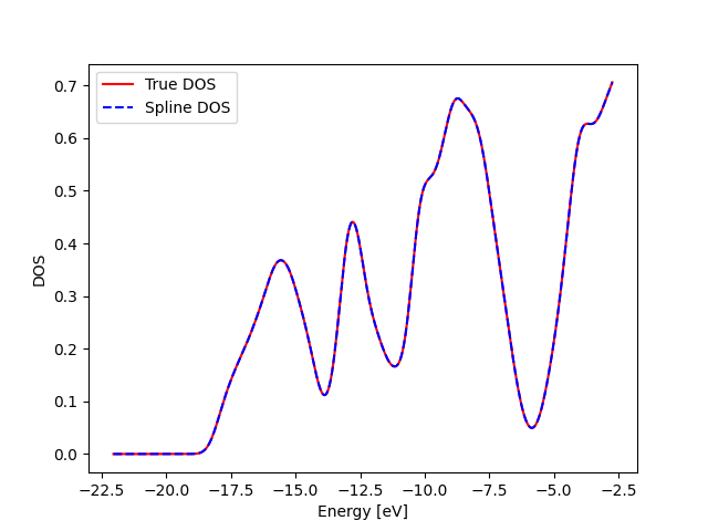
Both lines lie on each other
Test 2: Ability to reproduce the correct values at the shifted x_dos positions
shifts = torch.zeros(n_structures) + 0.3
x_dos_splines = x_dos_Ef + shifts.view(-1, 1)
spline_dos_Ef = evaluate_spline(total_splines_Ef, spline_positions_Ef, x_dos_splines)

plt.plot(x_dos_Ef, total_edos_Ef[0], color="red", label="True DOS")
plt.plot(x_dos_Ef, spline_dos_Ef[0], color="blue", linestyle="--", label="Spline DOS")
plt.legend()
plt.xlabel("Energy [eV]")
plt.ylabel("DOS")
print("Both spectras look very similar")
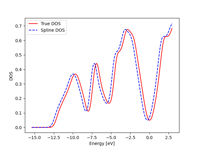
Both spectras look very similar
Step 2: Compute SOAP power spectrum for the dataset
We first define the hyperparameters to compute the SOAP power spectrum using featomic.
HYPER_PARAMETERS = {
    "cutoff": {"radius": 4.0, "smoothing": {"type": "Step"}},
    "density": {
        "type": "Gaussian",
        "width": 0.45,
        "scaling": {"type": "Willatt2018", "exponent": 5, "rate": 1, "scale": 3.0},
    },
    "basis": {
        "type": "TensorProduct",
        "max_angular": 6,
        "radial": {"type": "Gto", "max_radial": 7},
    },
}
We feed the Hyperparameters into featomic to compute the SOAP Power spectrum
calculator = SoapPowerSpectrum(**HYPER_PARAMETERS)
R_total_soap = calculator.compute(structures)
# Transform the tensormap to a single block containing a dense representation
R_total_soap.keys_to_samples("center_type")
R_total_soap.keys_to_properties(["neighbor_1_type", "neighbor_2_type"])

# Now we extract the data tensor from the single block
total_atom_soap = []
for structure_i in range(n_structures):
    a_i = R_total_soap.block(0).samples["system"] == structure_i
    total_atom_soap.append(torch.tensor(R_total_soap.block(0).values[a_i, :]))

total_soap = torch.stack(total_atom_soap)
Step 3: Building a Simple MLP Model
Split the data into Training, Validation and Test
Define the dataloader and the Model Architecture
Define relevant loss functions for training and inference
Define the training loop
Evaluate the model
1) Split the data into Training, Validation and Test
We will first split the data in a 7:1:2 manner, corresponding to train, val and test.
np.random.seed(0)
train_index = np.arange(n_structures)
np.random.shuffle(train_index)
test_mark = int(0.8 * n_structures)
val_mark = int(0.7 * n_structures)
test_index = train_index[test_mark:]
val_index = train_index[val_mark:test_mark]
train_index = train_index[:val_mark]
2) Define the dataloader and the Model Architecture
We will now build a dataloader and dataset to facillitate training the model batchwise
def generate_atomstructure_index(n_atoms_per_structure):
    """Generate a sequence of indices for each atom in the structure.
    The indices correspond to index of the structure that the atom belongs to

    Args:
        n_atoms_per_structure ([array]):
        [Array containing the number of atoms each structure contains]

    Return s:
        [tensor]: [Total index, matching atoms to structure]
    """
    # n_structures = len(n_atoms_per_structure)
    total_index = []
    for i, atoms in enumerate(n_atoms_per_structure):
        indiv_index = torch.zeros(atoms) + i
        total_index.append(indiv_index)
    total_index = torch.hstack(total_index)
    return total_index.long()


class AtomicDataset(Dataset):
    def __init__(self, features, n_atoms_per_structure):
        self.features = features
        self.n_structures = len(n_atoms_per_structure)
        self.n_atoms_per_structure = n_atoms_per_structure
        self.index = generate_atomstructure_index(self.n_atoms_per_structure)
        assert torch.sum(n_atoms_per_structure) == len(features)

    def __len__(self):
        return self.n_structures

    def __getitem__(self, idx):
        if isinstance(idx, list):  # If a list of indexes is given
            feature_indexes = []

            for i in idx:
                feature_indexes.append((self.index == i).nonzero(as_tuple=True)[0])

            feature_indexes = torch.hstack(feature_indexes)

            return (
                self.features[feature_indexes],
                idx,
                generate_atomstructure_index(self.n_atoms_per_structure[idx]),
            )

        else:
            feature_indexes = (self.index == idx).nonzero(as_tuple=True)[0]
            return (
                self.features[feature_indexes],
                idx,
                self.n_atoms_per_structure[idx],
            )


def collate(
    batch,
):  # Defines how to collate the outputs of the __getitem__ function at each batch
    for x, idx, index in batch:
        return (x, idx, index)


x_train = torch.flatten(total_soap[train_index], 0, 1).float()
total_atomic_soaps = torch.vstack(total_atom_soap).float()
train_features = AtomicDataset(x_train, n_atoms[train_index])
full_atomstructure_index = generate_atomstructure_index(n_atoms)
# Will be required later to collate atomic predictions into structural predictions

# Build a Dataloader that samples from the AtomicDataset in random batches
Sampler = RandomSampler(train_features)
BSampler = BatchSampler(Sampler, batch_size=32, drop_last=False)
traindata_loader = DataLoader(train_features, sampler=BSampler, collate_fn=collate)
We will now define a simple three layer MLP model, consisting of three layers. The align keyword is used to indicate that the energy reference will be optimized during training. The alignment parameter refers to the adjustments made to the initial energy referenced and will be initialized as zeros.
class SOAP_NN(torch.nn.Module):
    def __init__(self, input_dims, L1, n_train, target_dims, align):
        super(SOAP_NN, self).__init__()
        self.target_dims = target_dims
        self.fc1 = torch.nn.Linear(input_dims, L1)
        self.fc2 = torch.nn.Linear(L1, target_dims)
        self.silu = torch.nn.SiLU()
        self.align = align
        if align:
            initial_alignment = torch.zeros(n_train)
            self.alignment = torch.nn.parameter.Parameter(initial_alignment)

    def forward(self, x):
        result = self.fc1(x)
        result = self.silu(result)
        result = self.fc2(result)
        return result
We will use a small network architecture, whereby the input layer corresponds to the size of the SOAP features, 448, the intermediate layer corresponds to a tenth size of the input layer and the final layer corresponds to the number of outputs.
As a shorthand, the model that optimizes the energy reference during training will be called the alignment model
n_outputs_H = len(x_dos_H)
n_outputs_Ef = len(x_dos_Ef)


Model_H = SOAP_NN(
    x_train.shape[1],
    x_train.shape[1] // 10,
    len(train_index),
    n_outputs_H,
    align=False,
)
Model_Ef = SOAP_NN(
    x_train.shape[1],
    x_train.shape[1] // 10,
    len(train_index),
    n_outputs_Ef,
    align=False,
)
Model_Align = SOAP_NN(
    x_train.shape[1],
    x_train.shape[1] // 10,
    len(train_index),
    n_outputs_Ef,
    align=True,
)
# The alignment model takes the fermi level energy reference as the starting point
3) Define relevant loss functions for training and inference
We will now define some loss functions that will be useful when we implement the model training loop later and during model evaluation on the test set.
def t_get_mse(a, b, xdos):
    """Compute mean error between two Density of States.
    The mean error is integrated across the entire energy grid
    to provide a single value to characterize the error

    Args:
        a ([tensor]): [Predicted DOS]
        b ([tensor]): [True DOS]
        xdos ([tensor], optional): [Energy axis of DOS]

    Returns:
        [float]: [MSE]
    """
    if len(a.size()) > 1:
        mse = (torch.trapezoid((a - b) ** 2, xdos, axis=1)).mean()
    else:
        mse = (torch.trapezoid((a - b) ** 2, xdos, axis=0)).mean()
    return mse


def t_get_rmse(a, b, xdos):
    """Compute root mean squared error between two Density of States .

    Args:
        a ([tensor]): [Predicted DOS]
        b ([tensor]): [True DOS]
        xdos ([tensor], optional): [Energy axis of DOS]

    Raises:
        ValueError: [Occurs if tensor shapes are mismatched]

    Returns:
        [float]: [RMSE or %RMSE]
    """

    if len(a.size()) > 1:
        rmse = torch.sqrt((torch.trapezoid((a - b) ** 2, xdos, axis=1)).mean())
    else:
        rmse = torch.sqrt((torch.trapezoid((a - b) ** 2, xdos, axis=0)).mean())
    return rmse


def Opt_RMSE_spline(y_pred, xdos, target_splines, spline_positions, n_epochs):
    """Evaluates RMSE on the optimal shift of energy axis.
    The optimal shift is found via gradient descent after a gridsearch is performed.

    Args:
        y_pred ([tensor]): [Prediction/s of DOS]
        xdos ([tensor]): [Energy axis]
        target_splines ([tensor]): [Contains spline coefficients]
        spline_positions ([tensor]): [Contains spline positions]
        n_epochs ([int]): [Number of epochs to run for Gradient Descent]

    Returns:
        [rmse([float]), optimal_shift[tensor]]:
        [RMSE on optimal shift, the optimal shift itself]

    """
    optim_search_mse = []
    offsets = torch.arange(-2, 2, 0.1)
    # Grid-search is first done to reduce number of epochs needed for
    # gradient descent, typically 50 epochs will be sufficient
    # if searching within 0.1
    with torch.no_grad():
        for offset in offsets:
            shifts = torch.zeros(y_pred.shape[0]) + offset
            shifted_target = evaluate_spline(
                target_splines, spline_positions, xdos + shifts.view(-1, 1)
            )
            loss_i = ((y_pred - shifted_target) ** 2).mean(dim=1)
            optim_search_mse.append(loss_i)
        optim_search_mse = torch.vstack(optim_search_mse)
        min_index = torch.argmin(optim_search_mse, dim=0)
        optimal_offset = offsets[min_index]

    offset = optimal_offset

    shifts = torch.nn.parameter.Parameter(offset.float())
    opt_adam = torch.optim.Adam([shifts], lr=1e-2)
    best_error = torch.zeros(len(shifts)) + 100
    best_shifts = shifts.clone()
    for _ in range(n_epochs):
        shifted_target = evaluate_spline(
            target_splines, spline_positions, xdos + shifts.view(-1, 1)
        ).detach()

        def closure():
            opt_adam.zero_grad()
            shifted_target = evaluate_spline(
                target_splines, spline_positions, xdos + shifts.view(-1, 1)
            )
            loss_i = ((y_pred - shifted_target) ** 2).mean()
            loss_i.backward(gradient=torch.tensor(1), inputs=shifts)
            return loss_i

        opt_adam.step(closure)

        with torch.no_grad():
            each_loss = ((y_pred - shifted_target) ** 2).mean(dim=1).float()
            index = each_loss < best_error
            best_error[index] = each_loss[index].clone()
            best_shifts[index] = shifts[index].clone()

    # Evaluate

    optimal_shift = best_shifts
    shifted_target = evaluate_spline(
        target_splines, spline_positions, xdos + optimal_shift.view(-1, 1)
    )
    rmse = t_get_rmse(y_pred, shifted_target, xdos)
    return rmse, optimal_shift
4) Define the training loop
We will now define the model training loop, for simplicity we will only train each model for a fixed number of epochs, learning rate, and batch_size. The training and validation error at each epoch will be saved.
def train_model(model_to_train, fixed_DOS, structure_splines, spline_positions, x_dos):
    """Trains a model for 500 epochs

    Args:
        model_to_train ([torch.nn.Module]): [ML Model]
        fixed_DOS ([tensor]): [Contains the DOS at a fixed energy reference,
        useful for models that don't optimize the energy reference]
        structure_splines ([tensor]): [Contains spline coefficients]
        spline_positions ([tensor]): [Contains spline positions]
        x_dos ([tensor]): [Energy axis for the prediction]

    Returns:
        [train_loss_history([tensor]),
        val_loss_history[tensor],
        structure_results[tensor]]:

        [Respective loss histories and final structure predictions]
    """
    lr = 1e-2
    n_epochs = 500

    opt = torch.optim.Adam(model_to_train.parameters(), lr=lr)

    train_loss_history = []
    val_loss_history = []

    for _epoch in range(n_epochs):
        for x_data, idx, index in traindata_loader:
            opt.zero_grad()
            predictions = model_to_train.forward(x_data)
            structure_results = torch.zeros([len(idx), model_to_train.target_dims])
            # Sum atomic predictions in each structure
            structure_results = structure_results.index_add_(
                0, index, predictions
            ) / n_atoms[train_index[idx]].view(-1, 1)
            if model_to_train.align:
                alignment = model_to_train.alignment
                alignment = alignment - torch.mean(alignment)
                # Enforce that the alignments have a mean of zero since a constant
                # value across the dataset is meaningless when optimizing the
                # relative energy reference
                target = evaluate_spline(
                    structure_splines[train_index[idx]],
                    spline_positions,
                    x_dos + alignment[idx].view(-1, 1),
                )  # Shifts the target based on the alignment value
                pred_loss = t_get_mse(structure_results, target, x_dos)
                pred_loss.backward()
            else:
                pred_loss = t_get_mse(
                    structure_results, fixed_DOS[train_index[idx]], x_dos
                )
                pred_loss.backward()

            opt.step()
        with torch.no_grad():
            all_pred = model_to_train.forward(total_atomic_soaps.float())
            structure_results = torch.zeros([n_structures, model_to_train.target_dims])
            structure_results = structure_results.index_add_(
                0, full_atomstructure_index, all_pred
            ) / (n_atoms).view(-1, 1)
            if model_to_train.align:
                # Evaluate model on optimal shift as there is no information
                # regarding the shift from the fermi level energy reference
                # during inference

                alignment = model_to_train.alignment
                alignment = alignment - torch.mean(alignment)
                target = evaluate_spline(
                    structure_splines[train_index],
                    spline_positions,
                    x_dos + alignment.view(-1, 1),
                )

                train_loss = t_get_rmse(structure_results[train_index], target, x_dos)
                val_loss, val_shifts = Opt_RMSE_spline(
                    structure_results[val_index],
                    x_dos,
                    structure_splines[val_index],
                    spline_positions,
                    50,
                )

            else:
                train_loss = t_get_rmse(
                    structure_results[train_index], fixed_DOS[train_index], x_dos
                )
                val_loss = t_get_rmse(
                    structure_results[val_index], fixed_DOS[val_index], x_dos
                )

            train_loss_history.append(train_loss)
            val_loss_history.append(val_loss)
    train_loss_history = torch.tensor(train_loss_history)
    val_loss_history = torch.tensor(val_loss_history)
    return (
        train_loss_history,
        val_loss_history,
        structure_results,
    )
    # returns the loss history and the final set of predictions
H_trainloss, H_valloss, H_predictions = train_model(
    Model_H, total_edos_H, total_splines_H, spline_positions_H, x_dos_H
)

Ef_trainloss, Ef_valloss, Ef_predictions = train_model(
    Model_Ef, total_edos_Ef, total_splines_Ef, spline_positions_Ef, x_dos_Ef
)

Align_trainloss, Align_valloss, Align_predictions = train_model(
    Model_Align, total_edos_Ef, total_splines_Ef, spline_positions_Ef, x_dos_Ef
)
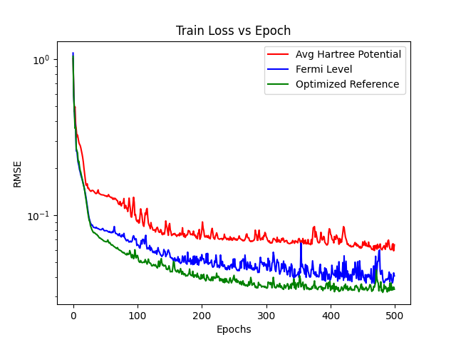
Lets plot the train loss histories to compare their learning behaviour
epochs = np.arange(500)


plt.plot(epochs, H_trainloss, color="red", label="Avg Hartree Potential")
plt.plot(epochs, Ef_trainloss, color="blue", label="Fermi Level")
plt.plot(epochs, Align_trainloss, color="green", label="Optimized Reference")
plt.legend()
plt.yscale(value="log")
plt.xlabel("Epochs")
plt.ylabel("RMSE")
plt.title("Train Loss vs Epoch")
plt.show()
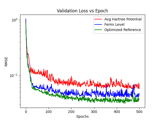
Lets plot the val loss histories to compare their learning behaviour
plt.plot(epochs, H_valloss, color="red", label="Avg Hartree Potential")
plt.plot(epochs, Ef_valloss, color="blue", label="Fermi Level")
plt.plot(epochs, Align_valloss, color="green", label="Optimized Reference")
plt.legend()
plt.yscale(value="log")
plt.xlabel("Epochs")
plt.ylabel("RMSE")
plt.title("Validation Loss vs Epoch")
plt.show()
5) Evaluate the model
We will now evaluate the model performance on the test set based on the model predictions we obtained previously
H_testloss = Opt_RMSE_spline(
    H_predictions[test_index],
    x_dos_H,
    total_splines_H[test_index],
    spline_positions_H,
    200,
)  # We use 200 epochs just so it the error a little bit more converged
Ef_testloss = Opt_RMSE_spline(
    Ef_predictions[test_index],
    x_dos_Ef,
    total_splines_Ef[test_index],
    spline_positions_Ef,
    200,
)  # We use 200 epochs just so it the error a little bit more converged
Align_testloss = Opt_RMSE_spline(
    Align_predictions[test_index],
    x_dos_Ef,
    total_splines_Ef[test_index],
    spline_positions_Ef,
    200,
)  # We use 200 epochs just so it the error a little bit more converged

print(f"Test RMSE for average Hartree Potential: {H_testloss[0].item():.3}")
print(f"Test RMSE for Fermi Level: {Ef_testloss[0].item():.3}")
print(f"Test RMSE for Optimized Reference: {Align_testloss[0].item():.3}")

print(
    "The difference in effectiveness between the Optimized Reference \
and the Fermi Level will increase with more epochs"
)
Test RMSE for average Hartree Potential: 0.0671
Test RMSE for Fermi Level: 0.0401
Test RMSE for Optimized Reference: 0.039
The difference in effectiveness between the Optimized Reference and the Fermi Level will increase with more epochs
Plot Training DOSes at different energy reference to visualize the impact of the energy reference. From the plots we can see that the optimized energy reference has better alignment of common spectral patterns across the dataset
Average Hartree Energy Reference
for i in total_edos_H[train_index]:
    plt.plot(x_dos_H, i, color="C0", alpha=0.6)
plt.title("Energy Reference - Average Hartree Potential")
plt.xlabel("Energy [eV]")
plt.ylabel("DOS")
plt.show()
print("The DOSes, despite looking similar, are offset along the energy axis")
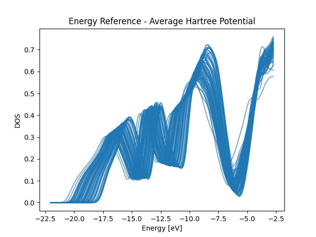
The DOSes, despite looking similar, are offset along the energy axis
Fermi Level Energy Reference
for i in total_edos_Ef[train_index]:
    plt.plot(x_dos_Ef, i, color="C0", alpha=0.6)
plt.title("Energy Reference - Fermi Level")
plt.xlabel("Energy [eV]")
plt.ylabel("DOS")
plt.show()

print("It is better aligned but still quite some offset")
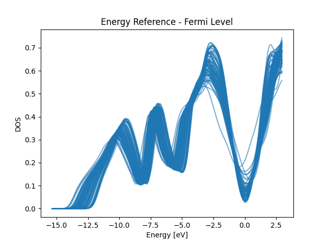
It is better aligned but still quite some offset
Optimized Energy Reference
shifts = Model_Align.alignment.detach()
shifts = shifts - torch.mean(shifts)
x_dos_splines = x_dos_Ef + shifts.view(-1, 1)
total_edos_align = evaluate_spline(
    total_splines_Ef[train_index], spline_positions_Ef, x_dos_splines
)

for i in total_edos_align:
    plt.plot(x_dos_Ef, i, color="C0", alpha=0.6)
plt.title("Energy Reference - Optimized")
plt.xlabel("Energy [eV]")
plt.ylabel("DOS")
plt.show()
print("The DOS alignment is better under the optimized energy reference")
print("The difference will increase with more training epochs")
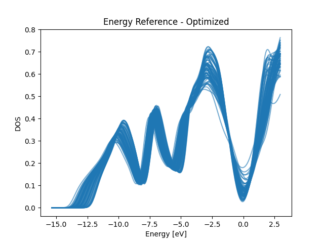
The DOS alignment is better under the optimized energy reference
The difference will increase with more training epochs
Total running time of the script: (1 minutes 27.505 seconds)