Multiple time stepping and ring-polymer contraction

Authors:

Davide Tisi @DavideTisi and Michele Ceriotti @ceriottm

This notebook provides an introduction to multiple time stepping and ring polymer contraction, two closely-related techniques, that are geared towards reducing the cost of calculations by separating slowly-varying (and computationally-expensive) components of the potential energy from the fast-varying (and hopefully cheaper) ones.

The first, multiple time stepping or MTS, is a well-established technique to avoid evaluating the slowly-varying components at every time step of a MD simulation. It was first introduced in M. Tuckerman, B. J. Berne, and G. J. Martyna, JCP 97(3), 1990 (1992) and can be applied to classical simulations, typically to avoid the evaluation of long-range electrostatics in classical empirical potentials.

The second, named ring polymer contraction, was first introduced in T. E. Markland and D. E. Manolopoulos, JCP 129(2), 024105 (2008) and can be seen as performing a similar simplification in imaginary time, evaluating the expensive part of the potential on a smaller number of PI replicas.

The techniques can be combined, which reduces even further the computational effort, which is the case we demonstrate in this notebook. This dual approach was introduced in V. Kapil, J. VandeVondele, and M. Ceriotti, JCP 144(5), 054111 (2016) and O. Marsalek and T. E. Markland, JCP 144(5), (2016). It is worth stressing that MTS and/or RPC can also be used very conveniently together with machine-learning potentials (see e.g. V. Kapil, J. Behler, and M. Ceriotti, JCP 145(23), 234103 (2016 or K. Rossi et al., JCTC 16(8), 5139 (2020) for early applications).

If you need an introduction to path integral simulations, or to the use of i-PI, which is the software which will be used to perform simulations, you can see this introductory recipe.

import os
import subprocess
import time
import warnings

import chemiscope
import ipi
import matplotlib.pyplot as plt
import numpy as np


if hasattr(__import__("builtins"), "get_ipython"):
    get_ipython().run_line_magic("matplotlib", "inline")  # noqa: F821

# sphinx_gallery_thumbnail_number = 2

Multiple time stepping in real and imaginary time

The core underlying assumption in these techniques is that the potential can be decomposed into a short-range/fast-varying/computationally-cheap part \(V_\mathrm{sr}\) and a long-range/slow-varying/computationally-expensive part \(V_\mathrm{lr}\). This is usually written as \(V=V_\mathrm{sr} +V_\mathrm{lr}\), although in many cases \(V_\mathrm{sr}\) is a cheap approximation of the potential, and \(V_\mathrm{lr}\) is taken to be the difference between this potential and the full one.

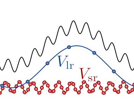
A smooth and rough potential components combine to form the total potential energy function used in a simulation.

The way this is realized in practice is by splitting the propagation of Hamilton’s equations into an inner loop that uses the fast/cheap force, and an outer loop that applies the slow force, using a larger time step (and therefore giving a larger “kick”).

\[\begin{split}\begin{split} &p \leftarrow p + f_\mathrm{lr} \, dt/2 \\ &\left. \begin{split} &p \leftarrow p + f_\mathrm{sr} \, dt/2M \\ &q \leftarrow q + p \, dt/M \\ &p \leftarrow p + f_\mathrm{sr} \, dt/2M \\ \end{split} \right\} M\ \mathrm{times}\\ &p \leftarrow p + f_\mathrm{lr} \, dt/2 \\ \end{split}\end{split}\]

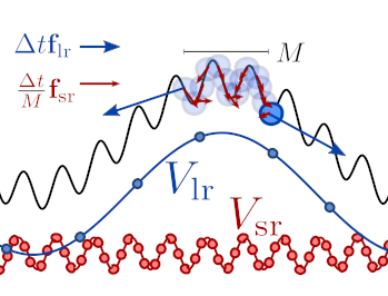
Schematic representation of the application of slow and fast forces in a multiple time step molecular dynamics algorithm

This approach can (and usually is) complemented by aggressive thermostatting, which helps stabilize the dynamics in the limit of large \(M\). For a detailed discussion on how thermostatting aids in this context, see: J. A. Morrone, T. E. Markland, M. Ceriotti, and B. J. Berne, JCP 134(1), 14103 (2011)

The idea behind ring-polymer contraction is very similar: it is unnecessary to evaluate on a very fine-grained discretization of the path integral components of the potential that are slowly-varying.

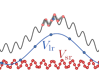
As shown in the figure below, ring-polymer contraction is realized by computing a Fourier interpolation of the bead positions, \(\tilde{\mathbf{q}}^{(k)}\), and then evaluating the total potential that enters the ring-polymer Hamiltonian as

\[V(\mathbf{q}) = \sum_{k=1}^P V_\mathrm{sr}(\mathbf{q}^{(k)}) + \frac{P}{P'} \sum_{k=1}^{P'} V_\mathrm{lr}(\tilde{\mathbf{q}}^{(k)})\]

where \(P\) and \(P'\) indicate the full and contracted discretizations of the path.

An example of the successive degrees of contraction of a ring polymer containing 16 beads (gray), interpolated down to 8 and 4.

A reference calculation using PIGLET

First, let’s run a reference calculation without RPC or MTS. These calculations will be performed using the q-TIP4P/f water model (S. Habershon, T. E. Markland, and D. E. Manolopoulos, JCP 131(2), 24501 (2009)) that contains a Morse-potential anharmonic intra-molecular potential, and an inter-molecular potential based on a Lennard-Jones term and a 4-point electrostatic model (the venerable TIP4P idea). It is fitted to reproduce experimental properties of water when performing PIMD calculations and it captures nicely several subtle effects while being cheap and easy-to-implement. The input for this run is h2o_pimd.xml, and we will use the -m qtip4pf option of i-pi-driver to compute the appropriate potential. To make simulations run quickly, we use a small box containing only 32 water molecules, and use a PIGLET thermostat that yields converged quantum properties with only 8 beads (cf. M. Ceriotti and D. E. Manolopoulos, Phys. Rev. Lett. 109(10), 100604 (2012), and also this introduction to the PIGLET method). For simplicity, we use the constant-volume NVT ensemble, but you can easily modify the input to perform constant-pressure simulations.

The important parts of the simulation - which we will modify to run a RPC/MTS simulation - are the definition of the forcefield socket

# Open and read the XML file
with open("data/h2o_pimd.xml", "r") as file:
    lines = file.readlines()

for line in lines[7:10]:
    print(line, end="")

<ffsocket mode='unix' name='qtip4pf' pbc='false'>
    <address>qtip4pf</address>
</ffsocket>

The important parts of the simulation - which we will modify to run a RPC/MTS simulation - are the definition of the forcefield socket, with the corresponding force definition

for line in lines[7:10]:
    print(line, end="")

print("\n[...]\n")

for line in lines[15:18]:
    print(line, end="")

  <ffsocket mode='unix' name='qtip4pf' pbc='false'>
      <address>qtip4pf</address>
  </ffsocket>

[...]

    <forces>
      <force forcefield='qtip4pf'/>
    </forces>

… the definition of the number of beads

print(lines[11], end="")

<initialize nbeads='8'>

… and the time step

print(lines[23], end="")

<timestep units='femtosecond'> 0.5 </timestep>

The <thermostat> section contains PIGLET parameters generated using the GLE4MD website .

Installing the Python driver

i-PI comes with a FORTRAN driver, which however has to be installed from source. We use a utility function to compile it. Note that this requires a functioning build system with gfortran and make.

ipi.install_driver()

Launch the i-PI simulation

We are going to launch i-PI from here, and put it in background and detach the processes from the jupyter instance, so we can continue with the notebook. On the the command line, this amounts to launching

PYTHONUNBUFFERED=1 i-pi data/h2o_pimd.xml &> log.pimd &
sleep 5
for i in `seq 1 4`; do
    i-pi-driver -u -a qtip4pf -m qtip4pf -v &> log.driver.$i &
done

From a Python script, one can launch both i-PI and the driver using the subprocess module:

ipi_process = None
if not os.path.exists("pimd.out"):
    ipi_process = subprocess.Popen(["i-pi", "data/h2o_pimd.xml"])
    time.sleep(5)  # wait for i-PI to start
    lmp_process = [
        subprocess.Popen(["i-pi-driver", "-u", "-a", "qtip4pf", "-m", "qtip4pf"])
        for i in range(4)
    ]

If you run this in a notebook, you can go ahead and start loading output files before i-PI and the driver have finished running, by skipping this cell

if ipi_process is not None:
    ipi_process.wait()
    for i in range(4):
        lmp_process[i].wait()

Multiple time stepping

Let’s now run a classical MD simulation, with and without multiple time stepping. We use very conservative parameters and a weak thermostat, to be able to see the difference in time scales between the full and short-range parts of the potential. Let’s first run a classical MD for reference. The input file is data/h2o_md.xml, nothing exciting to see there. The bash command this time would be:

PYTHONUNBUFFERED=1 i-pi data/h2o_md.xml &> log.md &
sleep 5
i-pi-driver -u -a qtip4pf-md -m qtip4pf -v &> log.driver.$i &

From Python:

ipi_process = None
if not os.path.exists("md.out"):
    ipi_process = subprocess.Popen(["i-pi", "data/h2o_md.xml"])
    time.sleep(5)  # wait for i-PI to start
    lmp_process = subprocess.Popen(
        ["i-pi-driver", "-u", "-a", "qtip4pf-md", "-m", "qtip4pf"]
    )

If you run this in a notebook, you can go ahead and start loading output files before i-PI and the driver have finished running, by skipping this cell

if ipi_process is not None:
    ipi_process.wait()
    lmp_process.wait()

Let’s have a look at h2o_mts.xml, that provides the parameters of the MTS calculation. We define two ffsocket sections: one will be used with the qtip4pf driver and the other with qtip4pf-sr. Note the different names of the sockets (that have to match the -a option in the invocation of the driver) and the internal labels that will be referred to in the <forces> section.

with open("data/h2o_mts.xml", "r") as file:
    lines = file.readlines()

for line in lines[7:13]:
    print(line, end="")

<ffsocket mode='unix' name='qtip4pf' pbc='false'>
    <address>qtip4pf-mts-full</address>
</ffsocket>
<ffsocket mode='unix' name='qtip4pf-sr' pbc='false'>
    <address>qtip4pf-mts-sr</address>
</ffsocket>

Each <force> block contains a <mts_weights> section. This provides a list of weights that determine which force components are active at each level of the MTS hierarchy. These weights indicate that the smooth part (full minus short-range) is active in the outer loop, and the short-range part is active in the inner loop. Note that the implementation is smart enough to re-use the short-range potential computed in the inner loop, multiplying it with a weight of -1 to compute \(V_\mathrm{lr}=V-V_\mathrm{sr}\).

for line in lines[18:26]:
    print(line, end="")

<forces>
  <force forcefield='qtip4pf'>
    <mts_weights>[1,0]</mts_weights>
  </force>
  <force forcefield='qtip4pf-sr'>
    <mts_weights>[-1,1]</mts_weights>
  </force>
</forces>

It remains to specify the MTS setup. We use an outer time step of 2 fs (four times the typical time step for room temperature water) and a splitting with M=4, so the fast forces are computed every 0.5 fs.

for line in lines[31:33]:
    print(line, end="")

<timestep units='femtosecond'> 2.0 </timestep>
<nmts>[1,4]</nmts>

One final detail, is that we print out the two components of the potential. This is achieved adding pot_component{units}(idx) to the <properties> field. The index corresponds to the order by which the <force> components are specified in the <forces> list. NB: the time step in i-PI is the outer time step, so it is not possible to access directly the value of the potential for intermediate inner steps

for line in lines[2]:
    print(line, end="")

<properties filename='out' stride='1'> [step, time{picosecond}, conserved{electronvolt}, temperature{kelvin}, potential{electronvolt}, kinetic_md{electronvolt}, pressure_md{megapascal}, pot_component{electronvolt}(0), pot_component{electronvolt}(1) ] </properties>

Let’s get the simulation going. Notice that we need two drivers, computing the short and full potentials, connected to the proper <ffsocket> on the i-PI side The correct bash command are:

PYTHONUNBUFFERED=1 i-pi data/h2o_mts.xml &> log.mts &
sleep 5
i-pi-driver -u -a qtip4pf-mts-full -m qtip4pf  &> log.driver.full &
i-pi-driver -u -a qtip4pf-mts-sr -m qtip4pf-sr &> log.driver.sr &
wait

that involve launching both short-range and full potential models. Similarly, in Python:

ipi_process = None
if not os.path.exists("mts.out"):
    ipi_process = subprocess.Popen(["i-pi", "data/h2o_mts.xml"])
    time.sleep(5)  # wait for i-PI to start
    lmp_process0 = subprocess.Popen(
        ["i-pi-driver", "-u", "-a", "qtip4pf-mts-full", "-m", "qtip4pf"]
    )
    lmp_process1 = subprocess.Popen(
        ["i-pi-driver", "-u", "-a", "qtip4pf-mts-sr", "-m", "qtip4pf-sr"]
    )

If you run this in a notebook, you can go ahead and start loading output files before i-PI and the drivers have finished running, by skipping this cell

if ipi_process is not None:
    ipi_process.wait()
    lmp_process0.wait()
    lmp_process1.wait()

Analysis of results

After having finished to run all simulation (might take a few minutes) we can load the outputs

md_output, md_desc = ipi.read_output("md.out")
mts_output, mts_desc = ipi.read_output("mts.out")

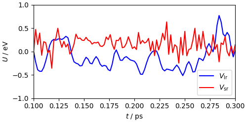
We can start looking at the behavior of the two components of the potential. Even though this is hardly the best slow/fast mode splitting (usually one also includes the Lennard-Jones and short-range Coulomb components in \(V_\mathrm{sr}\)) it is clear that the intra-molecular potential varies faster than the non-bonded components. Running the whole simulation with a 2 fs time step would lead to major instabilities in the trajectory.

fig, ax = plt.subplots(1, 1, constrained_layout=True, figsize=(5, 2.5))
ax.plot(
    mts_output["time"],
    mts_output["pot_component(0)"]
    - mts_output["pot_component(1)"]
    - (mts_output["pot_component(0)"] - mts_output["pot_component(1)"])[50],
    "b-",
    label=r"$V_\mathrm{lr}$",
)
ax.plot(
    mts_output["time"],
    mts_output["pot_component(1)"] - mts_output["pot_component(1)"][50],
    "r-",
    label=r"$V_\mathrm{sr}$",
)
ax.set_xlabel(r"$t$ / ps")
ax.set_ylabel(r"$U$ / eV")
ax.set_xlim(0.1, 0.3)
ax.set_ylim(-1, 1)
ax.legend()

<matplotlib.legend.Legend object at 0x7f7d1de69710>

This can be made clearer by computing the autocorrelation function, and seeing that the long-range term is that showing a slow decay, while the short-range one decays quickly to zero, rapidly oscillating

# a simple wrapper to np.correlate to evaluate the autocorrelation function
def autocorrelate(x, xbar=None, normalize=True):
    """Computes the autocorrelation function of a trajectory.
    It can be given the exact average as a parameter"""

    if xbar is None:
        xbar = x.mean()
    acf = np.correlate(x - xbar, x - xbar, mode="same")
    return acf[len(x) // 2 :] / (((x - xbar) * (x - xbar)).sum() if normalize else 1)


acf_vsr = autocorrelate(mts_output["pot_component(1)"][50:])
acf_vlr = autocorrelate(
    (mts_output["pot_component(0)"] - mts_output["pot_component(1)"])[50:]
)

fig, ax = plt.subplots(1, 1, constrained_layout=True, figsize=(5, 2.5))
ax.plot(
    mts_output["time"][: len(acf_vsr)],
    acf_vsr,
    "r-",
    label=r"$V_\mathrm{sr}$",
)
ax.plot(
    mts_output["time"][: len(acf_vlr)],
    acf_vlr,
    "b-",
    label=r"$V_\mathrm{lr}$",
)
ax.legend()
ax.set_xlabel(r"$t$ / ps")
ax.set_ylabel(r"$c_{VV}$")

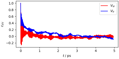
Text(18.567, 0.5, '$c_{VV}$')

The equilibration is slow due to the weak thermostat, but the two trajectories both equilibrate to 300 K. The difference in potential energy is not significant, because of the slow convergence of the potential energy in liquid water.

fig, ax = plt.subplots(1, 2, constrained_layout=True, figsize=(8, 3))
ax[1].plot(mts_output["time"], mts_output["potential"], "b-", label="MTS")
ax[1].plot(md_output["time"], md_output["potential"], "c.", label="MD")
ax[1].set_xlabel("t / ps")
ax[1].set_ylabel("U / eV")
ax[0].plot(mts_output["time"], mts_output["temperature"], "r-", label="MTS")
ax[0].plot(md_output["time"], md_output["temperature"], "m.", label="MD")
ax[0].set_xlabel("t / ps")
ax[0].set_ylabel("T / K")
ax[0].legend()
ax[1].legend()

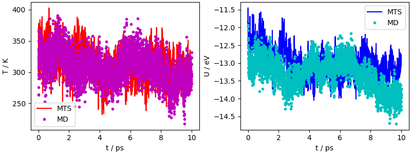
<matplotlib.legend.Legend object at 0x7f7d1d9f4990>

RPC/MTS simulation

Now let’s get to the full beast. The input for the RCP/MTS simulation is h2o_rpc-mts.xml. The setup is rather subtle, because we will use the F90 driver that implements the full q-TIP4P/f potential (with -m qtip4pf) and the intra-molecular part (with -m qtip4pf-sr). This means that we will have to compute the slowly-varying part as \(V_\mathrm{full}-V_\mathrm{sr}\). Let’s look at the key sections in the input file. Much as for the MTS setup, the simulation includes two ffsocket sections - one will be used with the qtip4pf driver and the other with qtip4pf-sr.

# Open and read the XML file
with open("data/h2o_rpc-mts.xml", "r") as file:
    lines = file.readlines()

for line in lines[7:13]:
    print(line, end="")

<ffsocket mode='unix' name='qtip4pf' pbc='false'>
    <address>qtip4pf-full</address>
</ffsocket>
<ffsocket mode='unix' name='qtip4pf-sr' pbc='false'>
    <address>qtip4pf-sr</address>
</ffsocket>

The <forces> section is where the magic happens. There are three components here. The first computes a full qtip4pf potential, and is computed on a contraction to 2 beads, as indicated by the nbeads=’2’ attribute. A second component is also evaluated on a contracted ring polymer, and is used to subtract the short-range component to leave the (smoother) long-range part. This is achieved linking to the qtip4pf-sr forcefield, and using the attribute weight=’-1’ to subtract the term from the total potential. Finally, there is another qtip4pf-sr component, that is evaluated on the full nbeads=’8’ ring polymer. The result is a RPC setup in which the smooth (Lennard-Jones + Coulomb) part of the potential is contracted on 2 replicas, and the fast part is computed on 8 replicas, which (thanks to the use of a PIGLET thermostat) is enough to achieve a good degree of convergence for water at 300 K.

Each <force> block also contains a <mts_weights> section, which is different from that used for the MTS simulation, because we now have a separate force component to subtract from the full potential, which is computed on the contracted ring polymer.

for line in lines[18:29]:
    print(line, end="")

<forces>
  <force forcefield='qtip4pf' nbeads='2'>
     <mts_weights>[1,0]</mts_weights>
  </force>
  <force forcefield='qtip4pf-sr' nbeads='2' weight='-1'>
     <mts_weights>[1,0]</mts_weights>
  </force>
  <force forcefield='qtip4pf-sr' nbeads='8'>
     <mts_weights>[0,1]</mts_weights>
  </force>
</forces>

It remains to specify the MTS setup. In this case, we use an outer time step of 1 fs (twice the typical time step for room temperature water) and a splitting with M=2, so the fast forces are computed every 0.5 fs. Compared to the classical MTS setup, we need a finer-grained integration because of the ring-polymer dynamics and because of the use of PIGLET, that requires a short time step to integrate accurately the Generalized Langevin equation. Still, even this splitting reduces by a factor of 2 the evaluations of the long-range potential.

for line in lines[34:36]:
    print(line, end="")

<timestep units='femtosecond'> 1.0 </timestep>
<nmts>[1,2]</nmts>

Finally, we are ready to run! We launch i-PI, and then execute two instances of the full potential (using -m qtip4pf and the correct socket address) and four instances of the short-range component, that is evaluated on the full ring polymer. This will take some time… The correct bash commands are:

PYTHONUNBUFFERED=1 i-pi h2o_rpc-mts.xml &> log.rpc-mts &
sleep 5
for i in `seq 1 2`; do
   i-pi-driver -u -a qtip4pf-full -m qtip4pf -v &> log.driver-full.$i &
done
for i in `seq 1 4`; do
   i-pi-driver -u -a qtip4pf-sr -m qtip4pf-sr -v &> log.driver-sr.$i &
done
wait

ipi_process = None
if not os.path.exists("rpc-mts.out"):
    ipi_process = subprocess.Popen(["i-pi", "data/h2o_rpc-mts.xml"])
    time.sleep(5)  # wait for i-PI to start
    lmp_process0 = [
        subprocess.Popen(["i-pi-driver", "-u", "-a", "qtip4pf-full", "-m", "qtip4pf"])
        for i in range(2)
    ]
    lmp_process1 = [
        subprocess.Popen(["i-pi-driver", "-u", "-a", "qtip4pf-sr", "-m", "qtip4pf-sr"])
        for i in range(4)
    ]

If you run this in a notebook, you can go ahead and start loading output files before i-PI and the drivers have finished running, by skipping this cell

if ipi_process is not None:
    ipi_process.wait()
    lmp_process0[0].wait()
    lmp_process0[1].wait()
    for i in range(4):
        lmp_process1[i].wait()

Analysis of results

Let’s read the results from the reference and RPC/MTS simulations and analyze them

pimd_output, pimd_desc = ipi.read_output("pimd.out")
rpcmts_output, rpcmts_desc = ipi.read_output("rpc-mts.out")

Let’s start looking at the long-range/contracted and short-range components of the potential. Here the long-range part is the sum of the first two components of the potential, since the second enters with a negative weight. We don’t see a clear time-scale separation here, because of the very aggressive PIGLET thermostat, that adds noise on top of the physical dynamics. This is not a major issue, because it only affects the dynamics of the momenta, but it means we cannot easily check for time scale separation when using advanced thermostatting schemes.

fig, ax = plt.subplots(1, 1, constrained_layout=True, figsize=(5, 2.5))
ax.plot(
    rpcmts_output["time"],
    (rpcmts_output["pot_component(0)"] - rpcmts_output["pot_component(1)"])
    - (rpcmts_output["pot_component(0)"] - rpcmts_output["pot_component(1)"])[10],
    "b-",
    label=r"$V_{\mathrm{lr}}$",
)
ax.plot(
    rpcmts_output["time"],
    rpcmts_output["pot_component(2)"] - rpcmts_output["pot_component(2)"][10],
    "r-",
    label=r"$V_{\mathrm{sr}}$",
)
ax.set_xlabel("t / ps")
ax.set_ylabel("U / eV")
ax.set_xlim(1.0, 1.5)
ax.set_ylim(-2, 2)
ax.legend()

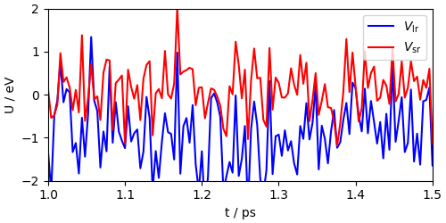
<matplotlib.legend.Legend object at 0x7f7d1da67dd0>

Simulations reach equilibrium faster than for the (weakly thermostatted) classical simulation, and even though the agreement between PIMD and the RPC+MTS run is not perfect, it is very good, in comparison with the major discrepancy between classical and quantum averages.

fig, ax = plt.subplots(1, 2, constrained_layout=True, figsize=(8, 3))
ax[0].plot(md_output["time"], md_output["potential"], "b-", label="MD")
ax[0].plot(pimd_output["time"], pimd_output["potential"], "r-", label="PIMD")
ax[0].plot(rpcmts_output["time"], rpcmts_output["potential"], "m.", label="RPC-MTS")
ax[0].set_xlabel("t / ps")
ax[0].set_ylabel("U / eV")
ax[1].plot(md_output["time"], md_output["kinetic_md"], "b-", label="MD")
ax[1].plot(pimd_output["time"], pimd_output["kinetic_cv"], "r-", label="PIMD")
ax[1].plot(rpcmts_output["time"], rpcmts_output["kinetic_cv"], "m.", label="RPC-MTS")
ax[1].set_xlabel("t / ps")
ax[1].set_ylabel("K / eV")
ax[0].set_xlim(0.0, 5.0)
ax[1].set_xlim(0.0, 5.0)
ax[0].legend()

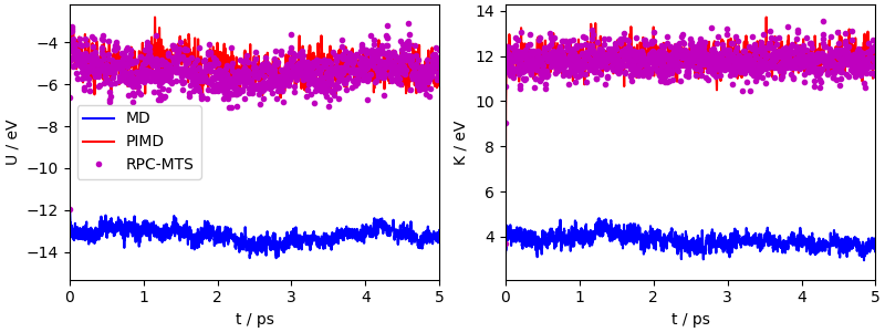
<matplotlib.legend.Legend object at 0x7f7d1d9a7050>

RPC+MTS simulations generate a distribution of structures at the highest path integral resolution, and can be used to compute all sorts of structural properties.

# loads structures, discarding unused atom properties
warnings.filterwarnings("ignore", ".*residuenumbers array.*")
pi_frames = [ipi.read_trajectory("rpc-mts.pos_" + str(i) + ".xyz") for i in range(8)]
frames = []
for idx_f in range(len(pi_frames[0])):
    f = pi_frames[0][idx_f]
    for k in range(1, 8):
        f += pi_frames[k][idx_f]
    f.info = {}
    f.arrays = {"positions": f.positions, "numbers": f.numbers}
    frames.append(f)


chemiscope.show(
    frames=frames,
    properties={
        "t": {
            "values": rpcmts_output["time"][::25],
            "units": "ps",
            "target": "structure",
        },
        "U": {
            "values": rpcmts_output["potential"][::25],
            "units": "eV",
            "target": "structure",
        },
        "K": {
            "values": rpcmts_output["kinetic_cv"][::25],
            "units": "eV",
            "target": "structure",
        },
    },
    settings=chemiscope.quick_settings(
        x="t",
        y="K",
        color="U",
        structure_settings={
            "bonds": False,
            "unitCell": True,
        },
        trajectory=True,
    ),
)

×