Path integral molecular dynamics

Authors:

Michele Ceriotti @ceriottm

This example shows how to run a path integral molecular dynamics simulation using i-PI, analyze the output and visualize the trajectory in chemiscope. It uses LAMMPS as the driver to simulate the q-TIP4P/f water model.

import os
import subprocess
import time

import ase.io
import chemiscope
import ipi
import matplotlib.pyplot as plt
import numpy as np
import upet
from atomistic_cookbook_utils import run_command
from huggingface_hub import hf_hub_download

Quantum nuclear effects and path integral methods

The Born-Oppenheimer approximation separates the joint quantum mechanical problem for electrons and nuclei into two independent problems. Even though often one makes the additional approximation of treating nuclei as classical particles, this is not necessary, and in some cases (typically when H atoms are present) can add considerable error.

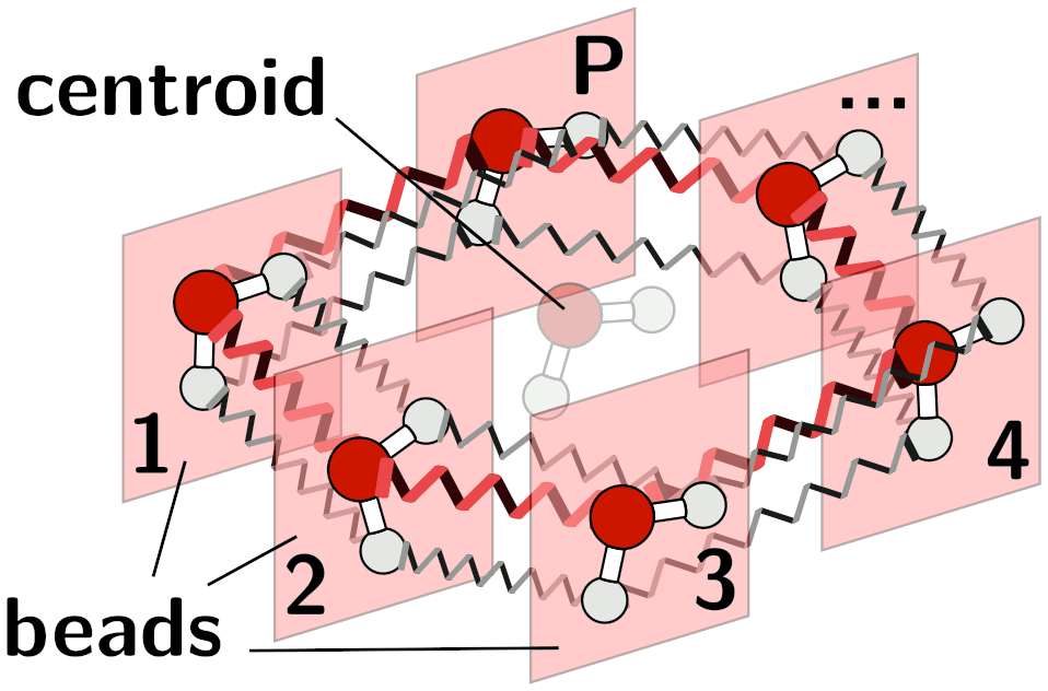
A representation of the ring-polymer Hamiltonian for a water molecule.

In order to describe the quantum mechanical nature of light nuclei (nuclear quantum effects) one of the most widely-applicable methods uses the path integral formalism to map the quantum partition function of a set of distinguishable particles onto the classical partition function of ring polymers composed by multiple beads (replicas) with corresponding atoms in adjacent replicas being connected by harmonic springs. The textbook by Tuckerman contains a pedagogic introduction to the topic, while this paper outlines the implementation used in i-PI.

The classical partition function of the path converges to quantum statistics in the limit of a large number of replicas. In this example, we will use a technique based on generalized Langevin dynamics, known as PIGLET to accelerate the convergence.

Running PIMD calculations with i-PI

i-PI is based on a client-server model, with i-PI controlling the nuclear dynamics (in this case sampling the path Hamiltonian using molecular dynamics) while the calculation of energies and forces is delegated to an external client program, in this example LAMMPS.

An i-PI calculation is specified by an XML file.

# Open and read the XML file
with open("data/input_pimd.xml", "r") as file:
    xml_content = file.read()
print(xml_content)

<simulation verbosity='medium' safe_stride='100'>
  <output prefix='simulation'>
    <properties stride='1' filename='out'>  [ step, time{picosecond}, conserved{electronvolt}, temperature{kelvin}, kinetic_cv{electronvolt}, potential{electronvolt}, pressure_cv{megapascal}, kinetic_td{electronvolt} ] </properties>
    <trajectory filename='pos' stride='20'> positions </trajectory>
    <trajectory filename='kin' stride='20'> kinetic_cv </trajectory>
    <trajectory filename='kod' stride='20'> kinetic_od </trajectory>
  </output>
  <total_steps> 200 </total_steps>
  <prng>
    <seed> 32342 </seed>
  </prng>
  <ffsocket name='lmpserial' mode='unix' pbc='false'>
      <address>h2o-lammps</address> <latency> 1e-4 </latency>
  </ffsocket>
  <system>
    <initialize nbeads='8'>
      <file mode='pdb' units='angstrom'> data/water_32.pdb </file>
      <velocities mode='thermal' units='kelvin'> 298 </velocities>
    </initialize>
    <forces>
      <force forcefield='lmpserial'> lmpserial </force>
    </forces>
    <ensemble>
      <temperature units='kelvin'>298</temperature>
    </ensemble>
    <motion mode='dynamics'>
      <dynamics mode='nvt'>
        <thermostat mode='pile_g'>
          <tau units="femtosecond"> 5.0 </tau>
        </thermostat>
        <timestep units='femtosecond'> 0.5 </timestep>
      </dynamics>
    </motion>
  </system>
</simulation>

NB1: In a realistic simulation you may want to increase the field total_steps, to simulate at least a few 100s of picoseconds.

NB2: To converge a simulation of water at room temperature, you typically need at least 32 beads. We will see later how to accelerate convergence using a colored-noise thermostat, but you can try to modify the input to check convergence with conventional PIMD

i-PI and lammps should be run separately, and it is possible to launch separate lammps processes to parallelize the evaluation over the beads. On the the command line, this amounts to launching

i-pi data/input_pimd.xml > log &
sleep 2
lmp -in data/in.lmp &
lmp -in data/in.lmp &

Note how i-PI and LAMMPS are completely independent, and therefore need a separate set of input files. The client-side communication in LAMMPS is described in the fix_ipi section, that matches the socket name and mode defined in the ffsocket field in the i-PI file.

We can launch the external processes from a Python script as follows

ipi_process = subprocess.Popen(["i-pi", "data/input_pimd.xml"])
time.sleep(2)  # wait for i-PI to start
lmp_process = [subprocess.Popen(["lmp", "-in", "data/in.lmp"]) for i in range(2)]

If you run this in a notebook, you can go ahead and start loading output files before i-PI and lammps have finished running, by skipping this cell

ipi_process.wait()
lmp_process[0].wait()
lmp_process[1].wait()

1

Analyzing the simulation

After the simulation has run, you can visualize and post-process the trajectory data. Note that i-PI prints a separate trajectory for each bead, as structural properties can be computed averaging over the configurations of any of the beads.

# drops first frame where all atoms overlap
output_data, output_desc = ipi.read_output("simulation.out")
traj_data = [ipi.read_trajectory(f"simulation.pos_{i}.xyz")[1:] for i in range(8)]

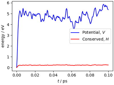
The simulation parameters are pushed at the limits: with the aggressive stochastic thermostatting and the high-frequency normal modes of the ring polymer, there are fairly large fluctuations of the conserved quantity. This is usually not affecting physical observables, but if you see this level of drift in a production run, check carefully for convergence and stability with a reduced time step.

fix, ax = plt.subplots(1, 1, figsize=(4, 3), constrained_layout=True)
ax.plot(
    output_data["time"],
    output_data["potential"] - output_data["potential"][0],
    "b-",
    label="Potential, $V$",
)
ax.plot(
    output_data["time"],
    output_data["conserved"] - output_data["conserved"][0],
    "r-",
    label="Conserved, $H$",
)
ax.set_xlabel(r"$t$ / ps")
ax.set_ylabel(r"energy / eV")
ax.legend()
plt.show()

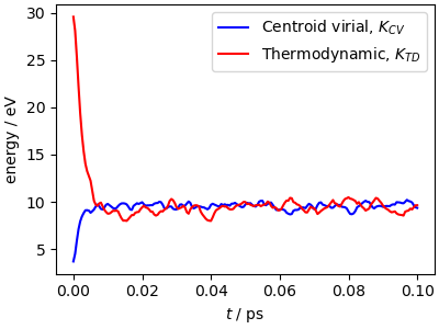
While the potential energy is simply the mean over the beads of the energy of individual replicas, computing the kinetic energy requires averaging special quantities that involve also the correlations between beads. Here we compare two of these estimators: the ‘thermodynamic’ estimator becomes statistically inefficient when increasing the number of beads, whereas the ‘centroid virial’ estimator remains well-behaved. Note how quickly these estimators equilibrate to roughly their stationary value, much faster than the equilibration of the potential energy above. This is thanks to the pile_g thermostat (see DOI:10.1063/1.3489925) that is optimally coupled to the normal modes of the ring polymer.

fix, ax = plt.subplots(1, 1, figsize=(4, 3), constrained_layout=True)
ax.plot(
    output_data["time"],
    output_data["kinetic_cv"],
    "b-",
    label="Centroid virial, $K_{CV}$",
)
ax.plot(
    output_data["time"],
    output_data["kinetic_td"],
    "r-",
    label="Thermodynamic, $K_{TD}$",
)
ax.set_xlabel(r"$t$ / ps")
ax.set_ylabel(r"energy / eV")
ax.legend()
plt.show()

You can also visualize the (very short) trajectory in a way that highlights the fast spreading out of the beads of the ring polymer. We use chemiscope’s ability to visualize custom shaped to interleave the trajectories of the beads, forming a trajectory that shows the connections between the replicas of each atom. Each atom and its connections are color-coded.

nbeads, nframes, natoms = (
    len(traj_data),
    len(traj_data[0]),
    len(traj_data[0][0]),
)

# creates frames with all beads, so we can use periodic boundary conditions when
# computing distances
full_frames = []
for i in range(nframes):
    struc = traj_data[0][i].copy()
    for k in range(1, nbeads):
        struc += traj_data[k][i]
    full_frames.append(struc)

distance_vectors = [
    full_frames[frame_i].get_distance(
        bead_i * natoms + atom_i,
        ((bead_i + 1) % nbeads) * natoms + atom_i,
        mic=True,
        vector=True,
    )
    for frame_i in range(nframes)
    for bead_i in range(nbeads)
    for atom_i in range(natoms)
]

paths_shapes = {
    "kind": "cylinder",
    "parameters": {
        "global": {"radius": 0.05},
        "atom": [{"vector": d.tolist()} for d in distance_vectors],
    },
}

properties = {
    "atom_id": [
        atom_i
        for frame_i in range(nframes)
        for bead_i in range(nbeads)
        for atom_i in range(natoms)
    ],
    "bead_id": [
        bead_i
        for frame_i in range(nframes)
        for bead_i in range(nbeads)
        for atom_i in range(natoms)
    ],
}

settings = {
    "structure": [
        {
            "atoms": False,
            "keepOrientation": True,
            "color": {"property": "bead_id", "palette": "hsv (periodic)"},
            "bonds": False,
            "shape": "paths",
            "environments": {"activated": False},
            "unitCell": True,
        }
    ]
}

chemiscope.show(
    full_frames,
    properties=properties,
    environments=chemiscope.all_atomic_environments(full_frames, 4.0),
    shapes={"paths": paths_shapes},
    mode="structure",
    settings=settings,
)

×

×

Accelerating PIMD with a PIGLET thermostat

The simulations in the previous sections are very far from converged – typically one would need approximately 32 replicas to converge a simulation of room-temperature water. To address this problem we will use a method based on generalized Langevin equations, called PIGLET

The input file is input_piglet.xml, that only differs by the definition of the thermostat, that uses a nm_gle mode in which each normal mode of the ring polymer is attached to a different colored-noise Generalized Langevin equation. This makes it possible to converge exactly the simulation results with a small number of replicas, and to accelerate greatly convergence for realistic systems such as this. The thermostat parameters can be generated on the GLE4MD website

ipi_process = subprocess.Popen(["i-pi", "data/input_piglet.xml"])
time.sleep(2)  # wait for i-PI to start
lmp_process = [subprocess.Popen(["lmp", "-in", "data/in.lmp"]) for i in range(2)]

ipi_process.wait()
lmp_process[0].wait()
lmp_process[1].wait()

1

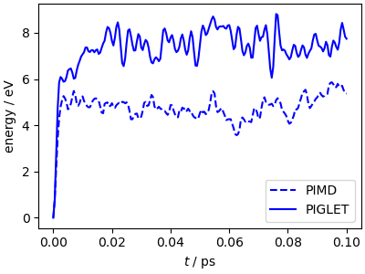
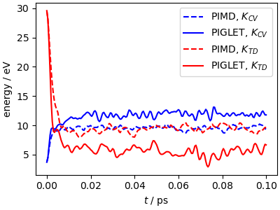
The mean potential energy from the PIGLET trajectory is higher than that for the PIMD one, because it is closer to the converged value (try to run a PIMD trajectory with 64 beads for comparison)

# drops first frame
output_gle, desc_gle = ipi.read_output("simulation_piglet.out")
traj_gle = [ipi.read_trajectory(f"simulation_piglet.pos_{i}.xyz")[1:] for i in range(8)]

fig, ax = plt.subplots(1, 1, figsize=(4, 3), constrained_layout=True)
ax.plot(
    output_data["time"],
    output_data["potential"] - output_data["potential"][0],
    "b--",
    label="PIMD",
)
ax.plot(
    output_gle["time"],
    output_gle["potential"] - output_gle["potential"][0],
    "b-",
    label="PIGLET",
)
ax.set_xlabel(r"$t$ / ps")
ax.set_ylabel(r"energy / eV")
ax.legend()
plt.show()

However, you should be somewhat careful: PIGLET converges some but not all the correlations within a path. For instance, it is designed to converge the centroid-virial estimator for the kinetic energy, but not the thermodynamic estimator. For the same reason, don’t try to look at equilibration in terms of the mean temperature: it won’t match the target value, because PIGLET uses a Langevin equation that breaks the classical fluctuation-dissipation theorem, and generates a steady-state distribution that mimics quantum fluctuations.

fix, ax = plt.subplots(1, 1, figsize=(4, 3), constrained_layout=True)
ax.plot(output_data["time"], output_data["kinetic_cv"], "b--", label="PIMD, $K_{CV}$")
ax.plot(output_gle["time"], output_gle["kinetic_cv"], "b", label="PIGLET, $K_{CV}$")
ax.plot(output_data["time"], output_data["kinetic_td"], "r--", label="PIMD, $K_{TD}$")
ax.plot(output_gle["time"], output_gle["kinetic_td"], "r", label="PIGLET, $K_{TD}$")
ax.set_xlabel(r"$t$ / ps")
ax.set_ylabel(r"energy / eV")
ax.legend()
plt.show()

Kinetic energy tensors

While we’re at it, let’s do something more complicated (and instructive). Classically, the momentum distribution of any atom is isotropic, so the kinetic energy tensor (KET) \(\mathbf{p}\mathbf{p}^T/2m\) is a constant times the identity matrix. Quantum mechanically, the kinetic energy tensor has more structure, that reflects the higher kinetic energy of particles along directions with stiff bonds. We can compute a moving average of the centroid virial estimator of the KET, and plot it to show the direction of anisotropy. Note that there are some subtleties connected with the evaluation of the moving average, see e.g. DOI:10.1103/PhysRevLett.109.100604

We first need to postprocess the components of the kinetic energy tensors (that i-PI prints out separating the diagonal and off-diagonal bits), averaging them over the last 10 frames and combining them with the centroid configuration from the last frame in the trajectory.

kinetic_cv = ipi.read_trajectory("simulation_piglet.kin.xyz")[1:]
kinetic_od = ipi.read_trajectory("simulation_piglet.kod.xyz")[1:]
kinetic_tens = np.hstack(
    [
        np.asarray([k.arrays["kinetic_cv"] for k in kinetic_cv[-10:]]).mean(axis=0),
        np.asarray([k.arrays["kinetic_od"] for k in kinetic_od[-10:]]).mean(axis=0),
    ]
)

centroid = traj_gle[-1][-1].copy()
centroid.positions = np.asarray([t[-1].positions for t in traj_gle]).mean(axis=0)
centroid.arrays["kinetic_cv"] = kinetic_tens

We can then view these in chemiscope, setting the proper parameters to visualize the ellipsoids associated with the KET. Note that some KETs have negative eigenvalues, because we are averaging over a few frames, which is insufficient to converge the estimator fully.

ellipsoids = chemiscope.ase_tensors_to_ellipsoids(
    [centroid], "kinetic_cv", scale=2, force_positive=True
)

chemiscope.show(
    [centroid],
    shapes={"kinetic_cv": ellipsoids},
    mode="structure",
    settings=chemiscope.quick_settings(
        structure_settings={
            "shape": ["kinetic_cv"],
            "unitCell": True,
        }
    ),
)

×

×

Path integrals with a machine-learning potential

The simulations above use an empirical forcefield, that describes the inter-atomic potential with a simple, fixed functional form. Machine-learning interatomic potentials, that are trained on electronic-structure calculations, approximate the Born-Oppenheimer potential energy surface, and therefore require an explicit treatment of nuclear quantum effects to model light atoms. Universal potentials, such as PET-MAD, are trained on databases that cover a large fraction of known compounds, and can therefore be applied, without further training, to systems beyond the reach of empirical models. As an example, we simulate a Li⁺ and an OH^- ion solvated in liquid water. We build the starting configuration by mutating two of the molecules in the water box used in the previous sections: one water is turned into Li⁺, and a second (distant) one loses a proton to become a hydroxide ion, so that the box stays charge-neutral.

atoms = ase.io.read("data/water_32.pdb")
# the box contains contiguous O,H,H triplets; the first molecule becomes Li+...
atoms.symbols[0] = "Li"
# ... deleting its two H atoms, together with one H of the 6th molecule (OH-)
del atoms[[1, 2, 16]]

# strips the PDB-specific arrays, and saves the structure keeping cell information
atoms = ase.Atoms(atoms.symbols, atoms.positions, cell=atoms.cell, pbc=True)
ase.io.write("water_lioh.xyz", atoms)

We use the extra-small version of PET-MAD, which is fast enough to run this example on CPU. We download the model checkpoint directly from the Hugging Face repository, and use the upet package to export it as a torchscript file.

model_path = "pet-mad-xs-v1.5.0.pt"
if not os.path.exists(model_path):
    checkpoint = hf_hub_download(
        repo_id="lab-cosmo/upet",
        filename="pet-mad-xs-v1.5.0.ckpt",
        subfolder="models",
    )
    upet.save_upet(checkpoint_path=checkpoint, output=model_path)

Warning: You are sending unauthenticated requests to the HF Hub. Please set a HF_TOKEN to enable higher rate limits and faster downloads.
/home/runner/work/atomistic-cookbook/atomistic-cookbook/.nox/path-integrals/lib/python3.12/site-packages/metatrain/pet/model.py:1428: UserWarning: the 'non_conservative_forces' output name is deprecated, please update the model to use 'non_conservative_force' instead
  return AtomisticModel(self.eval(), metadata, capabilities)
/home/runner/work/atomistic-cookbook/atomistic-cookbook/.nox/path-integrals/lib/python3.12/site-packages/metatrain/pet/model.py:1428: UserWarning: the 'non_conservative_forces' output name is deprecated, please update the model to use 'non_conservative_force' instead
  return AtomisticModel(self.eval(), metadata, capabilities)
/home/runner/work/atomistic-cookbook/atomistic-cookbook/.nox/path-integrals/lib/python3.12/site-packages/metatrain/llpr/model.py:999: UserWarning: the 'non_conservative_forces' output name is deprecated, please update the model to use 'non_conservative_force' instead
  return AtomisticModel(self.eval(), metadata, self.capabilities)

i-PI can evaluate the model directly, through the metatomic interface: rather than launching a separate driver connected by a socket, the input uses a ffdirect forcefield clause that computes energy and forces in the same process. Everything else in the input file – including the PIGLET thermostat, that is transferable between systems at the same temperature – is unchanged relative to the previous section.

with open("data/input_pet_piglet.xml", "r") as file:
    xml_content = file.read()
print(
    xml_content[
        xml_content.find("<ffdirect") : xml_content.find("</ffdirect>")
        + len("</ffdirect>")
    ]
)

run_command("i-pi data/input_pet_piglet.xml")

<ffdirect name='pet-mad'>
    <pes>metatomic</pes>
    <parameters> {template:water_lioh.xyz,model:pet-mad-xs-v1.5.0.pt,device:cpu,non_conservative:False} </parameters>
  </ffdirect>

CompletedProcess(args=['i-pi', 'data/input_pet_piglet.xml'], returncode=0)

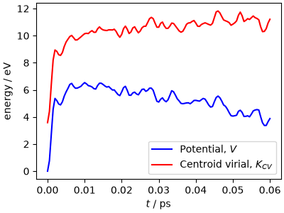
Even this very short trajectory shows the fast equilibration of the kinetic energy induced by the PIGLET thermostat.

output_pet, desc_pet = ipi.read_output("simulation_pet.out")

fig, ax = plt.subplots(1, 1, figsize=(4, 3), constrained_layout=True)
ax.plot(
    output_pet["time"],
    output_pet["potential"] - output_pet["potential"][0],
    "b-",
    label="Potential, $V$",
)
ax.plot(
    output_pet["time"],
    output_pet["kinetic_cv"],
    "r-",
    label="Centroid virial, $K_{CV}$",
)
ax.set_xlabel(r"$t$ / ps")
ax.set_ylabel(r"energy / eV")
ax.legend()
plt.show()

We visualize the ring polymers by simply superimposing the configurations of all the beads in each frame. Note the large spread of the beads of the protons compared with the compact ring polymer of the (heavier) Li⁺ ion, that is easy to spot given that atoms are colored by element.

traj_pet = [ipi.read_trajectory(f"simulation_pet.pos_{i}.xyz")[1:] for i in range(8)]
nbeads, nframes = len(traj_pet), len(traj_pet[0])

full_frames = []
for i in range(nframes):
    struc = traj_pet[0][i].copy()
    for k in range(1, nbeads):
        struc += traj_pet[k][i]
    full_frames.append(struc)

chemiscope.show(
    full_frames,
    mode="structure",
    settings=chemiscope.quick_settings(
        trajectory=True, structure_settings={"bonds": False, "unitCell": True}
    ),
)

×

×