Sample and Feature Selection with FPS and CUR

Authors:

Davide Tisi @DavideTisi and Hanna Tuerk @HannaTuerk

In this tutorial we generate descriptors using featomic, then select a subset of structures using both the farthest-point sampling (FPS) and CUR algorithms implemented in scikit-matter. Finally, we also generate a selection of the most important features using the same techniques.

First, import all the necessary packages

import os

import ase.io
import chemiscope
import metatensor
import numpy as np
import requests
from featomic import SoapPowerSpectrum
from matplotlib import pyplot as plt
from sklearn.decomposition import PCA
from skmatter import feature_selection, sample_selection


# Note that you will need a the specific new version of skmatter (state: Feb. 2025).
# The link is provided in the environment.yml file that you can find on github.

Load molecular data

Load 500 example BTO structures from file, reading them using ASE. The data is available as a download in the data.zip file below or in the atomistic-cookbook github.

filename = "gaas_training.xyz"
if not os.path.exists(filename):
    url = f"https://zenodo.org/records/10566825/files/{filename}"
    response = requests.get(url)
    response.raise_for_status()
    with open(filename, "wb") as f:
        f.write(response.content)

# Load a subset of `structures <data/input-fps.xyz>` of the example dataset
n_frames = 500
frames = ase.io.read("gaas_training.xyz", f":{3*n_frames}:3", format="extxyz")

Compute SOAP descriptors using featomic

First, define the featomic hyperparameters used to compute SOAP.

# featomic hyperparameters
hypers = {
    "cutoff": {"radius": 6.0, "smoothing": {"type": "ShiftedCosine", "width": 0.5}},
    "density": {
        "type": "Gaussian",
        "width": 0.3,
        "scaling": {"type": "Willatt2018", "exponent": 4, "rate": 1, "scale": 3.5},
    },
    "basis": {
        "type": "TensorProduct",
        "max_angular": 6,
        "radial": {"type": "Gto", "max_radial": 7},
    },
}

# Generate a SOAP power spectrum
calculator = SoapPowerSpectrum(**hypers)
rho2i = calculator.compute(frames)


# Makes a dense block
atom_soap = rho2i.keys_to_properties(["neighbor_1_type", "neighbor_2_type"])

atom_soap_single_block = atom_soap.keys_to_samples(keys_to_move=["center_type"])

# Sum over atomic centers to compute structure features
struct_soap = metatensor.sum_over_samples(
    atom_soap_single_block, sample_names=["atom", "center_type"]
)


print("atom feature descriptor shape:", atom_soap.block(0).values.shape)
print(
    "atom feature descriptor (all in one block) shape:",
    atom_soap_single_block.block(0).values.shape,
)
print("structure feature descriptor shape:", struct_soap.block(0).values.shape)

atom feature descriptor shape: (93670, 1344)
atom feature descriptor (all in one block) shape: (148821, 1344)
structure feature descriptor shape: (500, 1344)

Perform atomic environment (i.e. sample) selection

Using FPS and CUR algorithms, we can perform selection of atomic environments. These are implemented in skmatter which uses data stored in the metatensor format.

Suppose we want to select the 10 most diverse environments for each chemical species.

First, we can use the keys_to_properties operation in metatensor to move the neighbor species indices to the properties of the TensorBlocks. The resulting descriptor will be a TensorMap comprised of three blocks, one for each chemical species, where the chemical species indices are solely present in the keys.

print("----Atomic environment selection-----")

print(atom_soap)
print(atom_soap.block(0))

----Atomic environment selection-----
TensorMap with 2 blocks
keys: center_type
          31
          33
TensorBlock
    samples (93670): ['system', 'atom']
    components (): []
    properties (1344): ['neighbor_1_type', 'neighbor_2_type', 'l', 'n_1', 'n_2']
    gradients: None

select 10 atomic environments for each chemical species.

# Define the number of structures *per block* to select using FPS
n_envs = 10

# FPS sample selection
for key, block in atom_soap.items():
    sample_fps = sample_selection.FPS(n_to_select=n_envs, initialize="random").fit(
        atom_soap.block(key).values
    )
    sample_fps_idxs = sample_fps.selected_idx_

    # Print the selected envs for this block
    print("atomic envs selected with FPS:\n")

    selected_structures_idx = atom_soap.block(key).samples.values[sample_fps_idxs]
    newblock = metatensor.slice_block(block, axis="samples", selection=sample_fps_idxs)
    print("center_type:", key, "\n(struct_idx, atom_idx)\n", newblock.samples.values)

# CUR sample selection
for key, block in atom_soap.items():
    sample_cur = sample_selection.CUR(n_to_select=n_envs).fit(
        atom_soap.block(key).values
    )

    print("atomic envs selected with CUR:\n")
    newblock = metatensor.slice_block(
        block, axis="samples", selection=sample_cur.selected_idx_
    )
    print("center_type:", key, "\n(struct_idx, atom_idx)\n", newblock.samples.values)

atomic envs selected with FPS:

center_type: LabelsEntry(center_type=31)
(struct_idx, atom_idx)
 [[362  45]
 [118 103]
 [431 169]
 [301  84]
 [301 116]
 [ 24 224]
 [370 360]
 [314 134]
 [389 336]
 [423  38]]
atomic envs selected with FPS:

center_type: LabelsEntry(center_type=33)
(struct_idx, atom_idx)
 [[ 23 123]
 [311 147]
 [442  87]
 [161 288]
 [307 259]
 [174  89]
 [212 179]
 [224  73]
 [285 245]
 [398  46]]
atomic envs selected with CUR:

center_type: LabelsEntry(center_type=31)
(struct_idx, atom_idx)
 [[118 184]
 [ 24 156]
 [148 276]
 [ 75 131]
 [362 280]
 [295 232]
 [308 256]
 [235  59]
 [246 163]
 [236 312]]
atomic envs selected with CUR:

center_type: LabelsEntry(center_type=33)
(struct_idx, atom_idx)
 [[ 24 287]
 [ 16 288]
 [ 83  45]
 [ 75  95]
 [383 163]
 [306 322]
 [225 237]
 [174 183]
 [389  87]
 [140 179]]

Selecting from a combined pool of atomic environments

One can also select from a combined pool of atomic environments and structures, instead of selecting an equal number of atomic environments for each chemical species. In this case, we can move the ‘center_type’ key to samples such that our descriptor is a TensorMap consisting of a single block. Upon sample selection, the most diverse atomic environments will be selected, regardless of their chemical species.

print("----All atomic environment selection-----")

atom_soap_single_block = atom_soap.keys_to_samples(keys_to_move=["center_type"])
print("keys", atom_soap_single_block.keys)
print("blocks", atom_soap_single_block[0])
print("samples in first and only block", atom_soap_single_block[0].samples)

# Using the original SOAP descriptor, move all keys to properties.

# Define the number of structures to select using FPS
n_envs = 10

# FPS sample selection
sample_fps = sample_selection.FPS(n_to_select=n_envs, initialize="random").fit(
    atom_soap_single_block.block(0).values
)

sample_fps_idxs = sample_fps.selected_idx_
selected_structures_idxs = atom_soap_single_block.block(0).samples["system"][
    sample_fps_idxs
]
newblock = metatensor.slice_block(
    atom_soap_single_block.block(0), axis="samples", selection=sample_fps.selected_idx_
)

print(
    "atomic envs selected with FPS: \n (struct_idx, atom_idx, center_type) \n",
    newblock.samples.values,
)

----All atomic environment selection-----
keys Labels(
    _
    0
)
blocks TensorBlock
    samples (148821): ['system', 'atom', 'center_type']
    components (): []
    properties (1344): ['neighbor_1_type', 'neighbor_2_type', 'l', 'n_1', 'n_2']
    gradients: None
samples in first and only block Labels(
    system  atom  center_type
      0      0        31
      0      1        31
              ...
     499    358       31
     499    359       33
)
atomic envs selected with FPS:
 (struct_idx, atom_idx, center_type)
 [[146  49  31]
 [161 288  33]
 [311 147  33]
 [118  64  31]
 [431 169  31]
 [113 235  33]
 [  0 172  33]
 [ 24 224  31]
 [301 139  31]
 [100 289  33]]

Perform structure (i.e. sample) selection with FPS/CUR

Instead of atomic environments, one can also select diverse structures. We can use the sum_over_samples operation in metatensor to define features in the structural basis instead of the atomic basis. This is done by summing over the atomic environments, labeled by the ‘center’ index in the samples of the TensorMap.

Alternatively, one could use the mean_over_samples operation, depending on the specific inhomogeneity of the size of the structures in the training set.

print("----Structure selection-----")

struct_soap = metatensor.sum_over_samples(
    atom_soap_single_block, sample_names=["atom", "center_type"]
)

print("keys", struct_soap.keys)
print("blocks", struct_soap[0])
print("samples in first block", struct_soap[0].samples)

# Define the number of structures to select *per block* using FPS
n_structures = 10

# FPS structure selection
sample_fps = sample_selection.FPS(n_to_select=n_structures, initialize="random").fit(
    struct_soap.block(0).values
)
struct_fps_idxs = sample_fps.selected_idx_
print("structures selected with FPS:\n", sample_fps.selected_idx_)


# CUR structure selection
sample_cur = sample_selection.CUR(n_to_select=n_structures).fit(
    struct_soap.block(0).values
)

struct_cur_idxs = sample_cur.selected_idx_
print("structures selected with CUR:\n", struct_cur_idxs)

# Slice structure descriptor along axis 0 to contain only the selected structures
struct_soap_fps = struct_soap.block(0).values[struct_fps_idxs, :]
struct_soap_cur = struct_soap.block(0).values[struct_cur_idxs, :]
assert struct_soap_fps.shape == struct_soap_cur.shape

print("Structure descriptor shape before selection ", struct_soap.block(0).values.shape)
print("Structure descriptor shape after selection (FPS)", struct_soap_fps.shape)
print("Structure descriptor shape after selection (CUR)", struct_soap_cur.shape)

----Structure selection-----
keys Labels(
    _
    0
)
blocks TensorBlock
    samples (500): ['system']
    components (): []
    properties (1344): ['neighbor_1_type', 'neighbor_2_type', 'l', 'n_1', 'n_2']
    gradients: None
samples in first block Labels(
    system
      0
      1
     ...
     498
     499
)
structures selected with FPS:
 [172 224 235 160 488 317 375  24 403 472]
structures selected with CUR:
 [342 224 267 219 236 235 140 472  68 429]
Structure descriptor shape before selection  (500, 1344)
Structure descriptor shape after selection (FPS) (10, 1344)
Structure descriptor shape after selection (CUR) (10, 1344)

Visualize selected structures

sklearn can be used to perform PCA dimensionality reduction on the SOAP descriptors. The resulting PC coordinates can be used to visualize the the data alongside their structures in a chemiscope widget.

# Generate a structure PCA
struct_soap_pca = PCA(n_components=4).fit_transform(struct_soap.block(0).values)
assert struct_soap_pca.shape == (n_frames, 4)

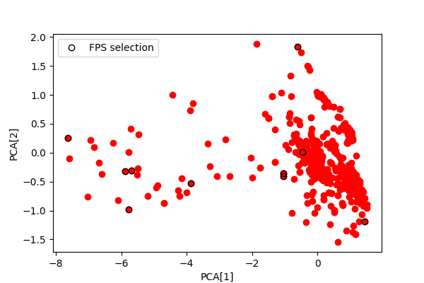
Plot the PCA map

Notice how the selected points avoid the densely-sampled area, and cover the periphery of the dataset

# Matplotlib plot
fig, ax = plt.subplots(1, 1, figsize=(6, 4))
scatter = ax.scatter(struct_soap_pca[:, 0], struct_soap_pca[:, 1], c="red")
ax.plot(
    struct_soap_pca[struct_cur_idxs, 0],
    struct_soap_pca[struct_cur_idxs, 1],
    "ko",
    fillstyle="none",
    label="FPS selection",
)
ax.set_xlabel("PCA[1]")
ax.set_ylabel("PCA[2]")
ax.legend()
fig.show()

Creates a chemiscope viewer

# Selected level
selection_levels = []
for i in range(len(frames)):
    level = 0
    if i in struct_cur_idxs:
        level += 1
    if i in struct_fps_idxs:
        level += 2
    if level == 0:
        level = "Not selected"
    elif level == 1:
        level = "CUR"
    elif level == 2:
        level = "FPS"
    else:
        level = "FPS+CUR"
    selection_levels.append(level)

properties = chemiscope.extract_properties(frames)

properties.update(
    {
        "PC1": struct_soap_pca[:, 0],
        "PC2": struct_soap_pca[:, 1],
        "PC3": struct_soap_pca[:, 2],
        "PC4": struct_soap_pca[:, 3],
        "selection": np.array(selection_levels),
    }
)

widget = chemiscope.show(
    frames,
    properties=properties,
    settings={
        "map": {
            "x": {"property": "PC1"},
            "y": {"property": "PC2"},
            "color": {"property": "energy"},
            "symbol": "selection",
            "size": {"factor": 50},
        },
        "structure": [{"unitCell": True}],
    },
)
widget.save("sample-selection.json.gz")

# display, if in notebook or sphinx
widget

×

Perform feature selection

Now perform feature selection to reduce the size of the features. In this example we will go back to using the descriptor decomposed into atomic environments, as opposed to the one decomposed into structure environments, but only use FPS for brevity.

print("----Feature selection-----")
print("keys", atom_soap_single_block.keys)
print("blocks", atom_soap_single_block[0])
print("samples in first block", atom_soap_single_block[0].properties)

# Define the number of features to select
n_features = 200

# FPS feature selection
feat_fps = feature_selection.FPS(n_to_select=n_features, initialize="random").fit(
    atom_soap_single_block.block(0).values
)
feat_fps_idxs = feat_fps.selected_idx_
atom_soap_single_block_fps = metatensor.slice_block(
    atom_soap_single_block.block(0), axis="properties", selection=feat_fps_idxs
)

# Slice atomic descriptor along axis 1 to contain only the selected features
print(
    "atomic descriptor shape before selection ",
    atom_soap_single_block.block(0).values.shape,
)
print(
    "atomic descriptor shape after selection ",
    atom_soap_single_block_fps.values.shape,
)

----Feature selection-----
keys Labels(
    _
    0
)
blocks TensorBlock
    samples (148821): ['system', 'atom', 'center_type']
    components (): []
    properties (1344): ['neighbor_1_type', 'neighbor_2_type', 'l', 'n_1', 'n_2']
    gradients: None
samples in first block Labels(
    neighbor_1_type  neighbor_2_type  l  n_1  n_2
          31               31         0   0    0
          31               31         0   0    1
                        ...
          33               33         6   7    6
          33               33         6   7    7
)
atomic descriptor shape before selection  (148821, 1344)
atomic descriptor shape after selection  (148821, 200)