Note
Go to the end to download the full example code.
Constant-temperature MD and thermostats
- Authors:
Michele Ceriotti @ceriottm
This recipe gives a practical introduction to finite-temperature molecular dynamics simulations, and provides a guide to choose the most appropriate thermostat for the simulation at hand.
As for other examples in the cookbook, a small simulation of liquid water is used as an archetypal example. Molecular dynamics, sampling, and constant-temperature simulations are discussed in much detail in the book “Understanding Molecular Simulations” by Daan Frenkel and Berend Smit. This seminal paper by H.C.Andersen provides a good historical introduction to the problem of thermostatting, and this PhD thesis provides a more detailed background to several of the techniques discussed in this recipe.
import os
import subprocess
import time
import xml.etree.ElementTree as ET

import chemiscope
import ipi
import matplotlib as mpl
import matplotlib.pyplot as plt
import numpy as np
from ipi.utils.tools.acf_xyz import compute_acf_xyz
from ipi.utils.tools.gle import get_gle_matrices, gle_frequency_kernel, isra_deconvolute
Constant-temperature sampling of (thermo)dynamics
Even though Hamilton’s equations in classical mechanics conserve the total energy of the group of atoms in a simulation, experimental boundary conditions usually involve exchange of heat with the surroundings, especially when considering the relatively small supercells that are often used in simulations.
The goal of a constant-temperature MD simulation is to compute efficiently thermal averages of the form \(\langle A(q,p)\rangle_\beta\), where the average of the observable \(A(q,p)\) is evaluated over the Boltzmann distribution at inverse temperature \(\beta=1/k_\mathrm{B}T\), \(P(q,p)=Q^{-1} \exp(-\beta(p^2/2m + V(q)))\) In all these scenarios, optimizing the simulation involves reducing as much as possible the autocorrelation time of the observable.
Constant-temperature sampling is also important when one wants to compute dynamical properties. In principle these would require constant-energy trajectories, as any thermostatting procedure modifies the dynamics of the system. However, the initial conditions should usually be determined from constant-temperature conditions, averaging over multiple constant-energy trajectories. As we shall see, this protocol can often be simplified greatly, by choosing thermostats that don’t interfere with the natural microscopic dynamics.
Running simulations
We use i-PI together with a LAMMPS driver to run
all the simulations in this recipe. The two codes need to be run separately,
and communicate atomic positions, energy and forces through a socket interface.
The LAMMPS input defines the parameters of the q-TIP4P/f water model, while the XML-formatted input of i-PI describes the setup of the MD simulation.
We begin running a constant-energy calculation, that
we will use to illustrate the metrics that can be applied to
assess the performance of a thermostatting scheme. If it is the
first time you see an i-PI input, you may want to look at
the input file side-by-sidewith the
input reference.
# Open and read the XML file
with open("data/input_nve.xml", "r") as file:
    xml_content = file.read()
print(xml_content)
<simulation verbosity='medium' safe_stride='100'>
  <output prefix='simulation_nve'>
      <properties stride='1' filename='out'>
      [ step, time{picosecond}, conserved{electronvolt},
      temperature{kelvin}, kinetic_md{electronvolt}, potential{electronvolt},
      temperature(H){kelvin}, temperature(O){kelvin} ] </properties>
    <trajectory filename='pos' stride='10'> positions </trajectory>
    <trajectory filename='vel' stride='1'> velocities </trajectory>
  </output>
  <total_steps> 2000 </total_steps>
  <prng>
    <seed> 32342 </seed>
  </prng>
  <ffsocket name='lmpserial' mode='unix' pbc='false'>
      <address>h2o-lammps</address> <latency> 1e-4 </latency>
  </ffsocket>
  <system>
    <initialize nbeads='1'>
      <file mode='pdb' units='angstrom'> data/water_32.pdb </file>
      <velocities mode='thermal' units='kelvin'> 300 </velocities>
    </initialize>
    <forces>
      <force forcefield='lmpserial'> lmpserial </force>
    </forces>
    <ensemble>
      <temperature units='kelvin'>300</temperature>
    </ensemble>
    <motion mode='dynamics'>
      <dynamics mode='nve'>
        <timestep units='femtosecond'> 1.0 </timestep>
      </dynamics>
    </motion>
  </system>
</simulation>
The part of the input that describes the molecular dynamics integrator
is the motion class. For this run, it specifies an NVE ensemble, and
a timestep of 1 fs for the integrator.
xmlroot = ET.parse("data/input_nve.xml").getroot()
print("    " + ET.tostring(xmlroot.find(".//motion"), encoding="unicode"))
<motion mode="dynamics">
  <dynamics mode="nve">
    <timestep units="femtosecond"> 1.0 </timestep>
  </dynamics>
</motion>
Note that this – and other runs in this example – are too short to
provide quantitative results, and you may want to increase the
<total_steps> parameter so that the simulation runs for at least
a few tens of ps. The time step of 1 fs is also at the limit of what
is acceptable for running simulations of water. 0.5 fs would be a
safer, stabler value.
To launch i-PI and LAMMPS from the command line you can just execute the following commands
i-pi data/input_nve.xml > log &
sleep 2
lmp -in data/in.lmp &
To launch the external processes from a Python script proceed as follows:
ipi_process = None
if not os.path.exists("simulation_nve.out"):
    ipi_process = subprocess.Popen(["i-pi", "data/input_nve.xml"])
    time.sleep(4)  # wait for i-PI to start
    lmp_process = [subprocess.Popen(["lmp", "-in", "data/in.lmp"]) for i in range(1)]
If you run this in a notebook, you can go ahead and start loading output files before i-PI and LAMMPS have finished running, by skipping this cell
if ipi_process is not None:
    ipi_process.wait()
    lmp_process[0].wait()
Analyzing the simulation
After the simulation is finished, we can look at the outputs. The outputs include the trajectory of positions, the velocities and a number of energetic observables
output_data, output_desc = ipi.read_output("simulation_nve.out")
traj_data = ipi.read_trajectory("simulation_nve.pos_0.xyz")
The trajectory shows mostly local vibrations on this short time scale,
but if you re-run with a longer <total_steps> settings you should be
able to observe diffusing molecules in the liquid.
chemiscope.show(
    traj_data,
    mode="structure",
    settings=chemiscope.quick_settings(
        trajectory=True, structure_settings={"unitCell": True}
    ),
)
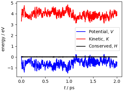
Potential and kinetic energy fluctuate, but the total energy is
(almost) constant, the small fluctuations being due to integration
errors, that are quite large with the long time step used for this
example. If you run with smaller <timestep> values, you should
see that the energy conservation condition is fulfilled with higher
accuracy.
fig, ax = plt.subplots(1, 1, figsize=(4, 3), constrained_layout=True)
ax.plot(
    output_data["time"],
    output_data["potential"] - output_data["potential"][0],
    "b-",
    label="Potential, $V$",
)
ax.plot(
    output_data["time"],
    output_data["kinetic_md"],
    "r-",
    label="Kinetic, $K$",
)
ax.plot(
    output_data["time"],
    output_data["conserved"] - output_data["conserved"][0],
    "k-",
    label="Conserved, $H$",
)
ax.set_xlabel(r"$t$ / ps")
ax.set_ylabel(r"energy / eV")
ax.legend()
plt.show()
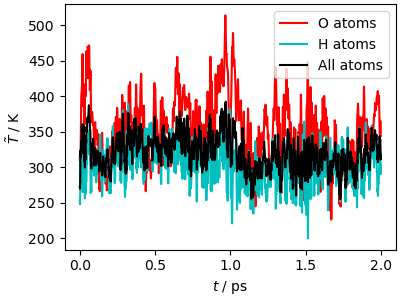
In a classical MD simulation, based on the momentum \(\mathbf{p}\) of each atom, it is possible to evaluate its kinetic temperature estimator \(T=\langle \mathbf{p}^2/m \rangle /3k_B\) the average is to be intended over a converged trajectory. Keep in mind that
The instantaneous value of this estimator is meaningless
It is only well-defined in a constant-temperature simulation, so here it only gives a sense of whether atomic momenta are close to what one would expect at 300 K.
With these caveats in mind, we can observe that the simulation has higher velocities than expected at 300 K, and that there is no equipartition, the O atoms having on average a higher energy than the H atoms.
fig, ax = plt.subplots(1, 1, figsize=(4, 3), constrained_layout=True)
ax.plot(
    output_data["time"],
    output_data["temperature(O)"],
    "r-",
    label="O atoms",
)
ax.plot(
    output_data["time"],
    output_data["temperature(H)"],
    "c-",
    label="H atoms",
)
ax.plot(output_data["time"], output_data["temperature"], "k-", label="All atoms")
ax.set_xlabel(r"$t$ / ps")
ax.set_ylabel(r"$\tilde{T}$ / K")
ax.legend()
plt.show()
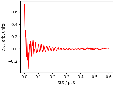
In order to investigate the dynamics more carefully, we
compute the velocity-velocity autocorrelation function
\(c_{vv}(t)=\sum_i \langle \mathbf{v}_i(t) \cdot \mathbf{v}_i(0) \rangle\).
We use a utility function that reads the outputs of i-PI
and computes both the autocorrelation function and its Fourier
transform.
\(c_{vv}(t)\) contains information on the time scale and amplitude
of molecular motion, and is closely related to the vibrational density
of states and to spectroscopic observables such as IR and Raman spectra.
acf_nve = compute_acf_xyz(
    "simulation_nve.vel_0.xyz",
    maximum_lag=600,
    length_zeropadding=2000,
    spectral_windowing="cosine-blackman",
    timestep=1,
    time_units="femtosecond",
    skip=100,
)

fig, ax = plt.subplots(1, 1, figsize=(4, 3), constrained_layout=True)
ax.plot(
    acf_nve[0][:1200] * 2.4188843e-05,  # atomic time to ps
    acf_nve[1][:1200] * 1e5,
    "r-",
)
ax.set_xlabel(r"$t$ / ps$")
ax.set_ylabel(r"$c_{vv}$ / arb. units")
plt.show()
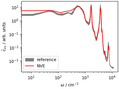
The power spectrum (that can be computed as the Fourier transform of
\(c_{vv}\)) reveals the frequencies of stretching, bending and libration
modes of water; the \(\omega\rightarrow 0\) limit is proportional
to the diffusion coefficient.
We also load the results from a reference calculation (average of 8
trajectories initiated from NVT-equilibrated samples, shown as the
confidence interval). You can see how to run these reference calculations
from the script data/run_traj.sh.
The differences are due to the short trajectory, and to the fact that the
NVE trajectory is not equilibrated at 300 K.
ha2cm1 = 219474.63

# Loads reference trajectory
acf_ref = np.loadtxt("data/traj-all_facf.data")

fig, ax = plt.subplots(1, 1, figsize=(4, 3), constrained_layout=True)

ax.fill_between(
    acf_ref[:1200, 0] * ha2cm1,
    (acf_ref[:1200, 1] - acf_ref[:1200, 2]) * 1e5,
    (acf_ref[:1200, 1] + acf_ref[:1200, 2]) * 1e5,
    color="gray",
    label="reference",
)

ax.loglog(acf_nve[3][:1200] * ha2cm1, acf_nve[4][:1200] * 1e5, "r-", label="NVE")
ax.set_xlabel(r"$\omega$ / cm$^{-1}$")
ax.set_ylabel(r"$\hat{c}_{vv}$ / arb. units")
ax.legend()
plt.show()
Langevin thermostatting
In order to perform a simulations that samples configurations consistent with a Boltzmann distribution \(e^{-V(x)/k_B T}\) one needs to modify the equations of motion. There are many different approaches to do this, some of which lead to deterministic dynamics; the two more widely used deterministic thermostats are the Berendsen thermostat which does not sample the Boltzmann distribution exactly and should never be used given the many more rigorous alternatives, and the Nosé-Hoover thermostat, that requires a “chain” implementation to be ergodic, which amounts essentially to a complicated way to generate poor-quality pseudo-random numbers.
Given the limitations of deterministic thermostats, in this recipe we focus on stochastic thermostats, that model the coupling to the chaotic dynamics of an external bath through explicit random numbers. Langevin dynamics amounts to adding to Hamilton’s equations of motion, for each degree of freedom, a term of the form
where :math:` gamma` is a friction coefficient, and \(\xi\) uncorrelated random numbers that mimic collisions with the bath particles. The friction can be seen as the inverse of a characteristic coupling time scale \(\tau=1/\gamma\) that describes how strongly the bath interacts with the system.
Setting up a thermostat in i-PI
In order to set up a thermostat in i-PI, one simply needs
to adjust the <dynamics> block, to perform nvt dynamics
and include an appropriate <thermostat> section.
Here we use a very-strongly coupled Langevin thermostat,
with \(\tau=10~fs\).
xmlroot = ET.parse("data/input_higamma.xml").getroot()
print("      " + ET.tostring(xmlroot.find(".//dynamics"), encoding="unicode"))
<dynamics mode="nvt">
  <timestep units="femtosecond"> 1.0 </timestep>
  <thermostat mode="langevin">
    <tau units="femtosecond"> 10 </tau>
  </thermostat>
</dynamics>
i-PI and LAMMPS are launched as above …
ipi_process = None
if not os.path.exists("simulation_higamma.out"):
    ipi_process = subprocess.Popen(["i-pi", "data/input_higamma.xml"])
    time.sleep(4)  # wait for i-PI to start
    lmp_process = [subprocess.Popen(["lmp", "-in", "data/in.lmp"]) for i in range(1)]
… and you should probably wait until they’re done, it’ll take less than a minute.
if ipi_process is not None:
    ipi_process.wait()
    lmp_process[0].wait()
Analysis of the trajectory
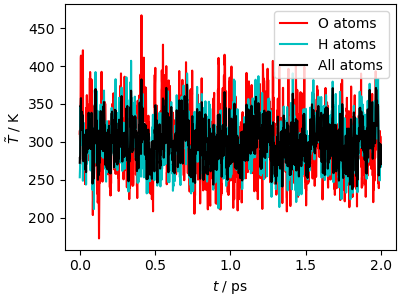
The temperature converges very quickly to the target value (fluctuations are to be expected, given that as discussed above the temperature estimator is just the instantaneous kinetic energy, that is not constant). There is also equipartition between O and H.
output_data, output_desc = ipi.read_output("simulation_higamma.out")
traj_data = ipi.read_trajectory("simulation_higamma.pos_0.xyz")

fig, ax = plt.subplots(1, 1, figsize=(4, 3), constrained_layout=True)
ax.plot(
    output_data["time"],
    output_data["temperature(O)"],
    "r-",
    label="O atoms",
)
ax.plot(
    output_data["time"],
    output_data["temperature(H)"],
    "c-",
    label="H atoms",
)
ax.plot(output_data["time"], output_data["temperature"], "k-", label="All atoms")
ax.set_xlabel(r"$t$ / ps")
ax.set_ylabel(r"$\tilde{T}$ / K")
ax.legend()
plt.show()
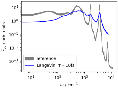
The velocity-velocity correlation function shows how much
this thermostat affects the system dynamics. The high-frequency peaks,
corresponding to stretches and bending, are
greatly broadened, and the \(\omega\rightarrow 0\)
limit of \(\hat{c}_{vv}\), corresponding to the
diffusion coefficient, is reduced by almost a factor of 5.
This last observation highlights that a too-aggressive
thermostat is not only disrupting the dynamics:
it also slows down diffusion through phase space,
making the dynamics less efficient at sampling slow,
collective motions. We shall see further down various
methods to counteract this effect, but in general one should
use a weaker coupling, that improves the sampling of configuration
space even though it slows down the convergence of the
kinetic energy. If you want a thermostat that equilibrates
aggressively the temperature while disturbing less the diffusive
modes, you may try the fast-forward Langevin thermostat
(Hijazi et al., JCP (2018))
that can be activated with the option mode="ffl".
# compute the v-v acf
acf_higamma = compute_acf_xyz(
    "simulation_higamma.vel_0.xyz",
    maximum_lag=600,
    length_zeropadding=2000,
    spectral_windowing="cosine-blackman",
    timestep=1,
    time_units="femtosecond",
    skip=100,
)

# and plot
fig, ax = plt.subplots(1, 1, figsize=(4, 3), constrained_layout=True)
ax.fill_between(
    acf_ref[:1200, 0] * ha2cm1,
    (acf_ref[:1200, 1] - acf_ref[:1200, 2]) * 1e5,
    (acf_ref[:1200, 1] + acf_ref[:1200, 2]) * 1e5,
    color="gray",
    label="reference",
)
ax.loglog(
    acf_higamma[3][:1200] * ha2cm1,
    acf_higamma[4][:1200] * 1e5,
    "b-",
    label=r"Langevin, $\tau=10$fs",
)
ax.set_xlabel(r"$\omega$ / cm$^{-1}$")
ax.set_ylabel(r"$\hat{c}_{vv}$ / arb. units")
ax.legend()
plt.show()
Global thermostats: stochastic velocity rescaling
An alternative approach to sample the canonical Boltzmann distribution while introducing fewer disturbances to the system dynamics is to use a global thermostat, i.e. a scheme that targets the total kinetic energy of the system, rather than that of individual degrees of freedom. We recommend the “stochastic velocity rescaling” thermostat (Bussi, Donadio, Parrinello, JCP (2007)) that acts by rescaling the total momentum vector, adding a suitably distributed random noise term.
Setting up a thermostat in i-PI
Stochastic velocity rescaling is implemented in i-PI
can be selected by setting mode="svr", and has a
tau parameter that corresponds to the time scale of the
coupling.
xmlroot = ET.parse("data/input_svr.xml").getroot()
print("        " + ET.tostring(xmlroot.find(".//thermostat"), encoding="unicode"))
<thermostat mode="svr">
  <tau units="femtosecond"> 10 </tau>
</thermostat>
We run a simulation with the usual set up …
ipi_process = None
if not os.path.exists("simulation_svr.out"):
    ipi_process = subprocess.Popen(["i-pi", "data/input_svr.xml"])
    time.sleep(4)  # wait for i-PI to start
    lmp_process = [subprocess.Popen(["lmp", "-in", "data/in.lmp"]) for i in range(1)]
… and wait for it to finish.
if ipi_process is not None:
    ipi_process.wait()
    lmp_process[0].wait()
Analysis of the trajectory
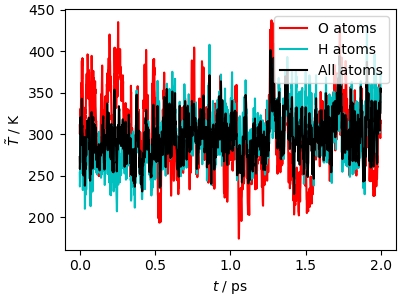
The kinetic temperature of the trajectory equilibrates very rapidly to the target value. However, it takes a bit longer (approximately 0.5 ps) to reach equipartition between O and H atoms. This is an important shortcoming of global thermostats: since they only target the total kinetic energy, they must rely on internal energy redistribution to reach equilibrium between different degrees of freedom. Liquid water is a very ergodic system, in which all degrees of freedom are strongly coupled, so this is not a major issue. However care must be taken when modeling a quasi-harmonic crystal (e.g. diamond, a metal, or an inorganic crystal), or a molecular system in which the coupling between molecules is weaker (e.g. methane, or another apolar compound).
output_data, output_desc = ipi.read_output("simulation_svr.out")
traj_data = ipi.read_trajectory("simulation_svr.pos_0.xyz")

fig, ax = plt.subplots(1, 1, figsize=(4, 3), constrained_layout=True)
ax.plot(
    output_data["time"],
    output_data["temperature(O)"],
    "r-",
    label="O atoms",
)
ax.plot(
    output_data["time"],
    output_data["temperature(H)"],
    "c-",
    label="H atoms",
)
ax.plot(output_data["time"], output_data["temperature"], "k-", label="All atoms")
ax.set_xlabel(r"$t$ / ps")
ax.set_ylabel(r"$\tilde{T}$ / K")
ax.legend()
plt.show()
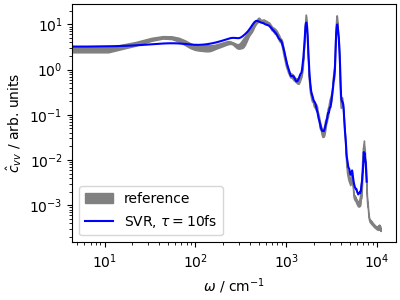
The velocity-velocity autocorrelation function is essentially indistinguishable from the reference, computed with an ensemble of NVE trajectories starting from canonical samples. In fact, the small discrepancies are mostly due to incomplete convergence of the averages in the short trajectory.
This highlights the advantages of a global thermostat, that does not disrupt the natural diffusion in configuration space, and can often be used to compute dynamical, time-dependent observables out of a single trajectory – which is far more practical than performing a collection of NVE trajectories.
acf_svr = compute_acf_xyz(
    "simulation_svr.vel_0.xyz",
    maximum_lag=600,
    length_zeropadding=2000,
    spectral_windowing="cosine-blackman",
    timestep=1,
    time_units="femtosecond",
    skip=100,
)

fig, ax = plt.subplots(1, 1, figsize=(4, 3), constrained_layout=True)
ax.fill_between(
    acf_ref[:1200, 0] * ha2cm1,
    (acf_ref[:1200, 1] - acf_ref[:1200, 2]) * 1e5,
    (acf_ref[:1200, 1] + acf_ref[:1200, 2]) * 1e5,
    color="gray",
    label="reference",
)
ax.loglog(
    acf_svr[3][:1200] * ha2cm1,
    acf_svr[4][:1200] * 1e5,
    "b-",
    label=r"SVR, $\tau=10$fs",
)
ax.set_xlabel(r"$\omega$ / cm$^{-1}$")
ax.set_ylabel(r"$\hat{c}_{vv}$ / arb. units")
ax.legend()
plt.show()
Generalized Langevin Equation thermostat
The issue with a Langevin thermostat is that, for a given coupling time \(\tau\), only molecular motions with a comparable time scale are sampled efficiently: faster modes are underdamped, and slower modes are overdamped, cf. the slowing down of diffusive behavior.
A possible solution to this problem is using a Generalized Langevin Equation (GLE) thermostat. A GLE thermostat uses a matrix generalization of the Langevin term, in which the physical momentum is supplemented by a few fictitious momenta \(\mathbf{s}\), i.e.
Here \(\mathbf{A}_p\) is the drift matrix and \(\mathbf{B}_p\) is a diffusion matrix which, for canonical sampling, is determined by the target temperature and the drift matrix through a fluctuation-dissipation relation. The key idea is that \(\mathbf{A}_p\) provides a lot of flexibility in defining the behavior of the GLE, that can be tuned to achieve near-optimal sampling for every degree of freedom (effectively acting as if the coupling constant was tuned separately for slow and fast molecular motions). The general idea and the practical implementation are discussed in (Ceriotti et al. JCTC (2010)) which also discusses other applications of the same principle, including performing simulations with a non-equilibrium quantum thermostat that mimics the quantum the quantum mechanical behavior of light nuclei.
Setting up a thermostat in i-PI
A GLE thermostat can be activated using mode="gle".
The drift matrix used here has been generated from the
GLE4MD website, using parameters that
aim for the most efficient sampling possible with the short
simulation time (2 ps). The online generator
can be tuned to provide the best possible sampling for the system
of interest, the most important parameter being the slowest time scale
that one is interested in sampling (typically a fraction of the total
simulation time). The range of frequencies that is optimized can then
be tuned so as to reach, roughly, the maximum frequency present in the
system.
xmlroot = ET.parse("data/input_gle.xml").getroot()
print("  " + ET.tostring(xmlroot.find(".//thermostat"), encoding="unicode"))
<thermostat mode="gle">
  <A shape="(7,7)">
    [   8.191023526179e-4,    8.328506066524e-3,    1.657771834013e-3,    9.736989925341e-4,    2.841803794895e-4,   -3.176846864198e-5,   -2.967010478210e-4,
-8.389856546341e-4,    2.405526974742e-2,   -1.507872374848e-2,    2.589784240185e-3,    1.516783633362e-3,   -5.958833418565e-4,    4.198422349789e-4,
 7.798710586406e-4,    1.507872374848e-2,    8.569039501219e-3,    6.001000899602e-3,    1.062029383877e-3,    1.093939147968e-3,   -2.661575532976e-3,
-9.676783161546e-4,   -2.589784240185e-3,   -6.001000899602e-3,    2.680459336535e-5,   -5.214694469742e-5,    4.231304910751e-4,   -2.104894919743e-5,
-2.841997149166e-4,   -1.516783633362e-3,   -1.062029383877e-3,    5.214694469742e-5,    1.433903506353e-9,   -4.241574212449e-5,    7.910178912362e-5,
 3.333208286893e-5,    5.958833418565e-4,   -1.093939147968e-3,   -4.231304910751e-4,    4.241574212449e-5,    2.385554468441e-8,   -3.139255482869e-5,
 2.967533789056e-4,   -4.198422349789e-4,    2.661575532976e-3,    2.104894919743e-5,   -7.910178912362e-5,    3.139255482869e-5,   2.432567259684e-11
   ]
  </A>
</thermostat>
We launch i-PI as usual …
ipi_process = None
if not os.path.exists("simulation_gle.out"):
    ipi_process = subprocess.Popen(["i-pi", "data/input_gle.xml"])
    time.sleep(4)  # wait for i-PI to start
    lmp_process = [subprocess.Popen(["lmp", "-in", "data/in.lmp"]) for i in range(1)]
… and wait for simulations to finish.
if ipi_process is not None:
    ipi_process.wait()
    lmp_process[0].wait()
Analysis of the trajectory
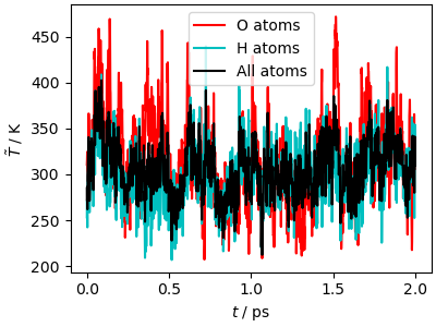
The kinetic temperature equilibrates quickly to the target value. Since the GLE is a local thermostat, targeting each degree of freedom separately, equipartition is also reached quickly. Sampling is less fast than with an aggressive Langevin thermostat, because the GLE targets each vibrational frequency separately, to minimize the impact on diffusion.
output_data, output_desc = ipi.read_output("simulation_gle.out")
traj_data = ipi.read_trajectory("simulation_gle.pos_0.xyz")

fig, ax = plt.subplots(1, 1, figsize=(4, 3), constrained_layout=True)
ax.plot(
    output_data["time"],
    output_data["temperature(O)"],
    "r-",
    label="O atoms",
)
ax.plot(
    output_data["time"],
    output_data["temperature(H)"],
    "c-",
    label="H atoms",
)
ax.plot(output_data["time"], output_data["temperature"], "k-", label="All atoms")
ax.set_xlabel(r"$t$ / ps")
ax.set_ylabel(r"$\tilde{T}$ / K")
ax.legend()
plt.show()
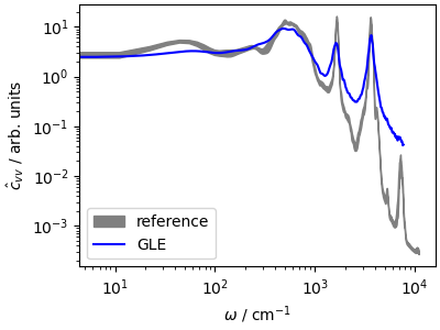
\(\hat{c}_{vv}\) reflects the adaptive behavior of the GLE. The fast modes are damped aggressively, leading to a large broadening of the high frequency peaks, but librations and diffusive modes are much less dampened than in the high-coupling Langevin case. An optimal-coupling GLE is a safe choice to sample any system, from molecular liquids to harmonic crystals, although a stochastic velocity rescaling is preferable if one is interested in preserving the natural dynamics.
acf_gle = compute_acf_xyz(
    "simulation_gle.vel_0.xyz",
    maximum_lag=600,
    length_zeropadding=2000,
    spectral_windowing="cosine-blackman",
    timestep=1,
    time_units="femtosecond",
    skip=100,
)

fig, ax = plt.subplots(1, 1, figsize=(4, 3), constrained_layout=True)
ax.fill_between(
    acf_ref[:1200, 0] * ha2cm1,
    (acf_ref[:1200, 1] - acf_ref[:1200, 2]) * 1e5,
    (acf_ref[:1200, 1] + acf_ref[:1200, 2]) * 1e5,
    color="gray",
    label="reference",
)
ax.loglog(
    acf_gle[3][:1200] * ha2cm1,
    acf_gle[4][:1200] * 1e5,
    "b-",
    label=r"GLE",
)
ax.set_xlabel(r"$\omega$ / cm$^{-1}$")
ax.set_ylabel(r"$\hat{c}_{vv}$ / arb. units")
ax.legend()
plt.show()
R-L purification
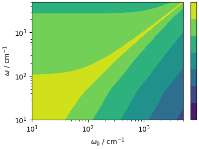
What if you also want to extract dynamical information from a GLE (or Langevin) trajectory? It is actually possible to post-process the power spectrum, performing a deconvolution based on the amount of disturbance introduced by the GLE, that can be predicted analytically in the harmonic limit. The idea, discussed in (Rossi et al., JCP (2018)) is that if \(\hat{y}(\omega)\) is the “natural” NVE power spectrum, and \(k_{\mathrm{GLE}}(\omega_0, \omega)\) is the power spectrum predicted for a harmonic oscillator of frequency \(\omega_0\), then the spectrum from the GLE dynamics will be approximately
The kernel can be computed analytically for all frequencies that
are relevant for the power spectrum, based on the GLE parameters
extracted from the input of i-PI.
n_omega = 1200
Ap, Cp, Dp = get_gle_matrices("data/input_gle.xml")
gle_kernel = gle_frequency_kernel(acf_gle[3][:n_omega], Ap, Dp)


lomega = acf_gle[3][:n_omega] * ha2cm1
fig, ax = plt.subplots(1, 1, figsize=(4, 3), constrained_layout=True)
levels = np.logspace(np.log10(gle_kernel.min()), np.log10(gle_kernel.max()), num=50)
contour = ax.contourf(lomega, lomega, gle_kernel, norm=mpl.colors.LogNorm())
ax.set_xscale("log")
ax.set_yscale("log")
ax.set_xlabel(r"$\omega_0$ / cm$^{-1}$")
ax.set_ylabel(r"$\omega$ / cm$^{-1}$")
ax.set_xlim(10, 5000)
ax.set_ylim(10, 5000)
cbar = fig.colorbar(contour, ticks=[1e1, 1e3, 1e5, 1e7])
 @system: Initializing system object
 @simulation: Initializing simulation object
@ RANDOM SEED: The seed used in this calculation was 32342
 @init_file: Initializing from file data/water_32.pdb. Dimension: length, units: angstrom, cell_units: automatic
 @init_file: Initializing from file data/water_32.pdb. Dimension: length, units: automatic, cell_units: automatic
 @init_file: Initializing from file data/water_32.pdb. Dimension: length, units: automatic, cell_units: automatic
 @init_file: Initializing from file data/water_32.pdb. Dimension: length, units: automatic, cell_units: automatic
 @init_file: Initializing from file data/water_32.pdb. Dimension: length, units: automatic, cell_units: automatic
 @initializer: Resampling velocities at temperature 300.0 kelvin
The deconvolution is based on the Iterative Image Space Reconstruction Algorithm, which preserves the positive-definiteness of the spectrum
isra_acf, history, errors, laplace = isra_deconvolute(
    acf_gle[3][:n_omega], acf_gle[4][:n_omega], gle_kernel, 64, 4
)
# error, laplacian =   2.003584422711218e-08, 5.5979243432528386e-11
# error, laplacian =   2.2056065682049772e-08, 1.7376959093763714e-10
# error, laplacian =   2.3108202455947157e-08, 4.097638626672861e-10
# error, laplacian =   2.3691949074988034e-08, 7.780596938258321e-10
# error, laplacian =   2.4035784182128285e-08, 1.2694751596779728e-09
# error, laplacian =   2.4249396569392062e-08, 1.861351757372963e-09
# error, laplacian =   2.4389091534014125e-08, 2.5265474789901312e-09
# error, laplacian =   2.4485088512215447e-08, 3.2391093879531283e-09
# error, laplacian =   2.455418992814817e-08, 3.976980779160915e-09
# error, laplacian =   2.460605884936594e-08, 4.722774066397663e-09
# error, laplacian =   2.464644566618402e-08, 5.463518998846859e-09
# error, laplacian =   2.4678890226455718e-08, 6.189986589300899e-09
# error, laplacian =   2.4705643657090066e-08, 6.8959202994722526e-09
# error, laplacian =   2.4728182632746304e-08, 7.577329137028943e-09
# error, laplacian =   2.4747505357273377e-08, 8.231898073229493e-09
Even though the ISRA algorithm is less prone to enhancing noise than other deconvolution algorithms, successive iterations sharpen the spectrum but introduce higher and higher levles of noise, particularly on the low-frequency end of the spectrum so one has to choose when to stop.
fig, ax = plt.subplots(1, 1, figsize=(4, 3), constrained_layout=True)
ax.loglog(
    acf_gle[3][:1200] * ha2cm1,
    acf_gle[4][:1200] * 1e5,
    "b-",
    label=r"GLE",
)
ax.loglog(
    acf_gle[3][:1200] * ha2cm1,
    history[0] * 1e5,
    ":",
    color="#4000D0",
    label=r"iter[1]",
)
ax.loglog(
    acf_gle[3][:1200] * ha2cm1,
    history[2] * 1e5,
    ":",
    color="#A000A0",
    label=r"iter[9]",
)
ax.loglog(
    acf_gle[3][:1200] * ha2cm1,
    history[4] * 1e5,
    ":",
    color="#D00040",
    label=r"iter[17]",
)
ax.loglog(
    acf_gle[3][:1200] * ha2cm1,
    history[12] * 1e5,
    ":",
    color="#FF0000",
    label=r"iter[49]",
)

ax.set_xlabel(r"$\omega$ / cm$^{-1}$")
ax.set_ylabel(r"$\hat{c}_{vv}$ / arb. units")
ax.legend()
plt.show()
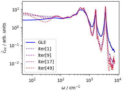
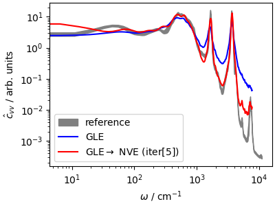
Especially in the high-frequency region, the deconvolution algorithm succeeds in recovering the underlying NVE dynamics, which can be useful whenever one wants to optimize statistical efficiency while still being able to estimate dynamical properties.
fig, ax = plt.subplots(1, 1, figsize=(4, 3), constrained_layout=True)
ax.fill_between(
    acf_ref[:1200, 0] * ha2cm1,
    (acf_ref[:1200, 1] - acf_ref[:1200, 2]) * 1e5,
    (acf_ref[:1200, 1] + acf_ref[:1200, 2]) * 1e5,
    color="gray",
    label="reference",
)
ax.loglog(
    acf_gle[3][:1200] * ha2cm1,
    acf_gle[4][:1200] * 1e5,
    "b-",
    label=r"GLE",
)
ax.loglog(
    acf_gle[3][:1200] * ha2cm1,
    history[2] * 1e5,
    "r-",
    label=r"GLE$\rightarrow$ NVE (iter[5])",
)
ax.set_xlabel(r"$\omega$ / cm$^{-1}$")
ax.set_ylabel(r"$\hat{c}_{vv}$ / arb. units")
ax.legend()
plt.show()
Running with LAMMPS
GLE thermostats (as well as conventional Langevin, and
stochastic velocity rescaling) are also implemented natively
in LAMMPS.
An example of LAMMPS input containing a GLE thermostat can
be found in data/gle.lmp. See also the
documentation of the fix gle command
fix 1 all gle 6 300 300 31415 data/smart.A
The drift matrix can be obtained from the same website, simply
asking to output the matrix in raw format, choosing units consistent
with the LAMMPS settings, e.g. for this optimal sampling setup
We can run LAMMPS from the command line
lmp -in data/gle.lmp &
or from Python
lmp_process = None
if not os.path.exists("lammps_out.dat"):
    lmp_process = subprocess.Popen(["lmp", "-in", "data/gle.lmp"])
… and wait
if lmp_process is not None:
    lmp_process.wait()
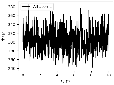
The simulation is much faster (for such a small system and
cheap potential the overhead of i-PI’s client-server mechanism
is substantial) and leads to similar results for the kinetic temperature
traj_data = np.loadtxt("lammps_out.dat")

fig, ax = plt.subplots(1, 1, figsize=(4, 3), constrained_layout=True)
ax.plot(
    traj_data[:, 0] * 1e-3,
    traj_data[:, 1],
    "k-",
    label="All atoms",
)
ax.set_xlabel(r"$t$ / ps")
ax.set_ylabel(r"$\tilde{T}$ / K")
ax.legend()
plt.show()
Total running time of the script: (1 minutes 17.771 seconds)