Note
Go to the end to download the full example code.
Learning Capabilities with torchpme
- Authors:
Egor Rumiantsev @E-Rum; Philip Loche @PicoCentauri
This example demonstrates the capabilities of the torchpme package, focusing on
learning target charges and utilizing the CombinedPotential class to evaluate
potentials that combine multiple pairwise interactions with optimizable weights.
The weights are optimized to reproduce the energy of a system interacting purely
through Coulomb forces.
import os
from typing import Dict

import ase.io
import ase.visualize.plot
import matplotlib.pyplot as plt
import numpy as np
import torch
from atomistic_cookbook_utils import download_with_retry
from torchpme import CombinedPotential, EwaldCalculator, InversePowerLawPotential
from vesin import NeighborList
Select computation device
device = "cpu"

if torch.cuda.is_available():
    device = "cuda"

dtype = torch.float32

prefactor = 0.5292  # Unit conversion prefactor.
Download and load the dataset
data_dir = "data"
dataset_url = "https://archive.materialscloud.org/records/405an-d8183/files/point_charges_Training_set_p1.xyz"  # noqa: E501
dataset_path = os.path.join(data_dir, "point_charges_Training_set.xyz")

download_with_retry(dataset_url, dataset_path)

# The dataset consists of atomic configurations with reference energies.
frames = ase.io.read(dataset_path, ":10")
Define model parameters
cell = frames[0].get_cell().array
cell_dimensions = np.linalg.norm(cell, axis=1)
cutoff = np.min(cell_dimensions) / 2 - 1e-6  # Define the cutoff distance.
smearing = cutoff / 6.0  # Smearing parameter for interaction potentials.
lr_wavelength = 0.5 * smearing  # Wavelength for long-range interactions.

params = {"lr_wavelength": lr_wavelength}
Build the neighbor list
The neighbor list is used to identify interacting pairs within the cutoff distance.
nl = NeighborList(cutoff=cutoff, full_list=False)

l_positions = []
l_cell = []
l_neighbor_indices = []
l_neighbor_distances = []
l_ref_energy = torch.zeros(len(frames), device=device, dtype=dtype)

for i_atoms, atoms in enumerate(frames):
    # Compute neighbor indices and distances
    i, j, d = nl.compute(
        points=atoms.positions, box=atoms.cell.array, periodic=True, quantities="ijd"
    )
    i = torch.from_numpy(i.astype(int))
    j = torch.from_numpy(j.astype(int))

    # Store atom positions, cell information, neighbor indices, and distances
    l_positions.append(torch.tensor(atoms.positions, device=device, dtype=dtype))
    l_cell.append(torch.tensor(atoms.cell.array, device=device, dtype=dtype))
    l_neighbor_indices.append(torch.vstack([i, j]).to(device=device).T)
    l_neighbor_distances.append(torch.from_numpy(d).to(device=device, dtype=dtype))

    # Store reference energy
    l_ref_energy[i_atoms] = torch.tensor(
        atoms.get_potential_energy(), device=device, dtype=dtype
    )
Function to assign charges to atoms
def assign_charges(atoms, charge_dict: Dict[str, torch.Tensor]) -> torch.Tensor:
    """Assign charges to atoms based on their chemical symbols."""
    chemical_symbols = np.array(atoms.get_chemical_symbols())
    charges = torch.zeros(len(atoms), dtype=dtype, device=device)

    for chemical_symbol, charge in charge_dict.items():
        charges[chemical_symbols == chemical_symbol] = charge

    return charges.reshape(-1, 1)
Define the energy computation
def compute_energy(charge_dict: Dict[str, torch.Tensor]) -> torch.Tensor:
    """Compute the total energy based on assigned charges and potentials."""
    energy = torch.zeros(len(frames), device=device, dtype=dtype)
    for i_atoms, atoms in enumerate(frames):
        charges = assign_charges(atoms, charge_dict)

        potential = calculator(
            charges=charges,
            cell=l_cell[i_atoms],
            positions=l_positions[i_atoms],
            neighbor_indices=l_neighbor_indices[i_atoms],
            neighbor_distances=l_neighbor_distances[i_atoms],
        )
        energy[i_atoms] = (charges * potential).sum()

    return energy
Define the loss function
def loss(charge_dict: Dict[str, torch.Tensor]) -> torch.Tensor:
    """Calculate the loss as the mean squared error between computed and reference
    energies."""
    energy = compute_energy(charge_dict)
    mse = torch.sum((energy - l_ref_energy) ** 2)

    return mse.sum()  # Optionally add charge_penalty for strict neutrality enforcement.
Fit charge model
Set initial values for the potential
potential = CombinedPotential(
    potentials=[
        InversePowerLawPotential(exponent=1.0, smearing=smearing, prefactor=prefactor)
    ],
    smearing=smearing,
)
calculator = EwaldCalculator(potential=potential, **params)
calculator.to(device=device, dtype=dtype)

q_Na = torch.tensor(1e-5).to(device=device, dtype=dtype)
q_Na.requires_grad = True

q_Cl = -torch.tensor(1e-5 + 0.2).to(device=device, dtype=dtype)
q_Cl.requires_grad = True

charge_dict = {"Na": q_Na, "Cl": q_Cl}
Learning loop: optimize charges to minimize the loss function
optimizer = torch.optim.Adam([q_Na, q_Cl], lr=0.1)

q_Na_timeseries = []
q_Cl_timeseries = []
loss_timeseries = []

for step in range(1000):
    optimizer.zero_grad()

    charge_dict = {"Na": q_Na, "Cl": q_Cl}

    loss_value = loss(charge_dict)
    loss_value.backward()
    optimizer.step()

    if step % 10 == 0:
        print(
            f"Step: {step:>5}, Loss: {loss_value.item():>5.2e}, "
            + ", ".join([f"q_{k}: {v:>5.2f}" for k, v in charge_dict.items()]),
            end="\r",
        )

    loss_timeseries.append(float(loss_value.detach().cpu()))
    q_Na_timeseries.append(float(q_Na.detach().cpu()))
    q_Cl_timeseries.append(float(q_Cl.detach().cpu()))

    if loss_value < 1e-10:
        break
Step:     0, Loss: 4.78e+01, q_Na: -0.10, q_Cl: -0.30
Step:    10, Loss: 8.50e+00, q_Na: -0.48, q_Cl: -0.73
Step:    20, Loss: 6.67e+00, q_Na: -0.42, q_Cl: -0.75
Step:    30, Loss: 6.34e+00, q_Na: -0.35, q_Cl: -0.76
Step:    40, Loss: 6.28e+00, q_Na: -0.34, q_Cl: -0.85
Step:    50, Loss: 5.86e+00, q_Na: -0.23, q_Cl: -0.87
Step:    60, Loss: 5.22e+00, q_Na: -0.13, q_Cl: -0.95
Step:    70, Loss: 4.31e+00, q_Na:  0.02, q_Cl: -1.04
Step:    80, Loss: 2.95e+00, q_Na:  0.24, q_Cl: -1.12
Step:    90, Loss: 1.46e+00, q_Na:  0.50, q_Cl: -1.18
Step:   100, Loss: 4.43e-01, q_Na:  0.74, q_Cl: -1.16
Step:   110, Loss: 8.37e-02, q_Na:  0.90, q_Cl: -1.09
Step:   120, Loss: 6.79e-03, q_Na:  0.97, q_Cl: -1.03
Step:   130, Loss: 7.23e-05, q_Na:  1.00, q_Cl: -0.99
Step:   140, Loss: 1.50e-03, q_Na:  1.01, q_Cl: -0.98
Step:   150, Loss: 1.61e-03, q_Na:  1.01, q_Cl: -0.98
Step:   160, Loss: 9.30e-04, q_Na:  1.01, q_Cl: -0.99
Step:   170, Loss: 3.59e-04, q_Na:  1.01, q_Cl: -0.99
Step:   180, Loss: 9.25e-05, q_Na:  1.00, q_Cl: -1.00
Step:   190, Loss: 1.25e-05, q_Na:  1.00, q_Cl: -1.00
Step:   200, Loss: 1.08e-07, q_Na:  1.00, q_Cl: -1.00
Step:   210, Loss: 8.58e-07, q_Na:  1.00, q_Cl: -1.00
Step:   220, Loss: 1.18e-06, q_Na:  1.00, q_Cl: -1.00
Step:   230, Loss: 6.38e-07, q_Na:  1.00, q_Cl: -1.00
Step:   240, Loss: 1.93e-07, q_Na:  1.00, q_Cl: -1.00
Step:   250, Loss: 2.80e-08, q_Na:  1.00, q_Cl: -1.00
Step:   260, Loss: 3.72e-10, q_Na:  1.00, q_Cl: -1.00
Step:   270, Loss: 2.19e-09, q_Na:  1.00, q_Cl: -1.00
Step:   280, Loss: 2.74e-09, q_Na:  1.00, q_Cl: -1.00
Step:   290, Loss: 1.28e-09, q_Na:  1.00, q_Cl: -1.00
Step:   300, Loss: 4.12e-10, q_Na:  1.00, q_Cl: -1.00
Step:   310, Loss: 1.70e-10, q_Na:  1.00, q_Cl: -1.00
Step:   320, Loss: 1.70e-10, q_Na:  1.00, q_Cl: -1.00
Step:   330, Loss: 1.76e-10, q_Na:  1.00, q_Cl: -1.00
Step:   340, Loss: 1.64e-10, q_Na:  1.00, q_Cl: -1.00
Step:   350, Loss: 1.67e-10, q_Na:  1.00, q_Cl: -1.00
Step:   360, Loss: 1.67e-10, q_Na:  1.00, q_Cl: -1.00
Step:   370, Loss: 1.75e-10, q_Na:  1.00, q_Cl: -1.00
Step:   380, Loss: 1.67e-10, q_Na:  1.00, q_Cl: -1.00
Step:   390, Loss: 1.75e-10, q_Na:  1.00, q_Cl: -1.00
Step:   400, Loss: 1.75e-10, q_Na:  1.00, q_Cl: -1.00
Step:   410, Loss: 1.67e-10, q_Na:  1.00, q_Cl: -1.00
Step:   420, Loss: 1.75e-10, q_Na:  1.00, q_Cl: -1.00
Step:   430, Loss: 1.67e-10, q_Na:  1.00, q_Cl: -1.00
Step:   440, Loss: 1.75e-10, q_Na:  1.00, q_Cl: -1.00
Step:   450, Loss: 1.67e-10, q_Na:  1.00, q_Cl: -1.00
Step:   460, Loss: 1.67e-10, q_Na:  1.00, q_Cl: -1.00
Step:   470, Loss: 1.75e-10, q_Na:  1.00, q_Cl: -1.00
Step:   480, Loss: 1.67e-10, q_Na:  1.00, q_Cl: -1.00
Step:   490, Loss: 1.75e-10, q_Na:  1.00, q_Cl: -1.00
Step:   500, Loss: 1.67e-10, q_Na:  1.00, q_Cl: -1.00
Step:   510, Loss: 1.75e-10, q_Na:  1.00, q_Cl: -1.00
Step:   520, Loss: 1.67e-10, q_Na:  1.00, q_Cl: -1.00
Step:   530, Loss: 1.75e-10, q_Na:  1.00, q_Cl: -1.00
Step:   540, Loss: 1.67e-10, q_Na:  1.00, q_Cl: -1.00
Step:   550, Loss: 1.75e-10, q_Na:  1.00, q_Cl: -1.00
Step:   560, Loss: 1.67e-10, q_Na:  1.00, q_Cl: -1.00
Step:   570, Loss: 1.75e-10, q_Na:  1.00, q_Cl: -1.00
Step:   580, Loss: 1.67e-10, q_Na:  1.00, q_Cl: -1.00
Step:   590, Loss: 1.75e-10, q_Na:  1.00, q_Cl: -1.00
Step:   600, Loss: 1.67e-10, q_Na:  1.00, q_Cl: -1.00
Step:   610, Loss: 1.75e-10, q_Na:  1.00, q_Cl: -1.00
Step:   620, Loss: 1.67e-10, q_Na:  1.00, q_Cl: -1.00
Step:   630, Loss: 1.75e-10, q_Na:  1.00, q_Cl: -1.00
Step:   640, Loss: 1.75e-10, q_Na:  1.00, q_Cl: -1.00
Step:   650, Loss: 1.67e-10, q_Na:  1.00, q_Cl: -1.00
Step:   660, Loss: 1.75e-10, q_Na:  1.00, q_Cl: -1.00
Step:   670, Loss: 1.67e-10, q_Na:  1.00, q_Cl: -1.00
Step:   680, Loss: 1.75e-10, q_Na:  1.00, q_Cl: -1.00
Step:   690, Loss: 1.75e-10, q_Na:  1.00, q_Cl: -1.00
Step:   700, Loss: 1.67e-10, q_Na:  1.00, q_Cl: -1.00
Step:   710, Loss: 1.75e-10, q_Na:  1.00, q_Cl: -1.00
Step:   720, Loss: 1.67e-10, q_Na:  1.00, q_Cl: -1.00
Step:   730, Loss: 1.75e-10, q_Na:  1.00, q_Cl: -1.00
Step:   740, Loss: 1.75e-10, q_Na:  1.00, q_Cl: -1.00
Step:   750, Loss: 1.67e-10, q_Na:  1.00, q_Cl: -1.00
Step:   760, Loss: 1.75e-10, q_Na:  1.00, q_Cl: -1.00
Step:   770, Loss: 1.67e-10, q_Na:  1.00, q_Cl: -1.00
Step:   780, Loss: 1.67e-10, q_Na:  1.00, q_Cl: -1.00
Step:   790, Loss: 1.75e-10, q_Na:  1.00, q_Cl: -1.00
Step:   800, Loss: 1.67e-10, q_Na:  1.00, q_Cl: -1.00
Step:   810, Loss: 1.67e-10, q_Na:  1.00, q_Cl: -1.00
Step:   820, Loss: 1.75e-10, q_Na:  1.00, q_Cl: -1.00
Step:   830, Loss: 1.67e-10, q_Na:  1.00, q_Cl: -1.00
Step:   840, Loss: 1.67e-10, q_Na:  1.00, q_Cl: -1.00
Step:   850, Loss: 1.75e-10, q_Na:  1.00, q_Cl: -1.00
Step:   860, Loss: 1.75e-10, q_Na:  1.00, q_Cl: -1.00
Step:   870, Loss: 1.67e-10, q_Na:  1.00, q_Cl: -1.00
Step:   880, Loss: 1.75e-10, q_Na:  1.00, q_Cl: -1.00
Step:   890, Loss: 1.75e-10, q_Na:  1.00, q_Cl: -1.00
Step:   900, Loss: 1.67e-10, q_Na:  1.00, q_Cl: -1.00
Step:   910, Loss: 1.57e-10, q_Na:  1.00, q_Cl: -1.00
Step:   920, Loss: 1.57e-10, q_Na:  1.00, q_Cl: -1.00
Step:   930, Loss: 1.57e-10, q_Na:  1.00, q_Cl: -1.00
Step:   940, Loss: 1.57e-10, q_Na:  1.00, q_Cl: -1.00
Step:   950, Loss: 1.67e-10, q_Na:  1.00, q_Cl: -1.00
Step:   960, Loss: 1.75e-10, q_Na:  1.00, q_Cl: -1.00
Step:   970, Loss: 1.75e-10, q_Na:  1.00, q_Cl: -1.00
Step:   980, Loss: 1.67e-10, q_Na:  1.00, q_Cl: -1.00
Step:   990, Loss: 1.67e-10, q_Na:  1.00, q_Cl: -1.00
Fit kernel model
The second phase involves optimizing the weights of the combined potential kernels.
Set initial values for the kernel model
potential = CombinedPotential(
    [
        InversePowerLawPotential(exponent=1.0, smearing=smearing, prefactor=prefactor),
        InversePowerLawPotential(exponent=2.0, smearing=smearing, prefactor=prefactor),
    ],
    smearing=smearing,
)

calculator = EwaldCalculator(potential=potential, **params)
calculator.to(device=device, dtype=dtype)
EwaldCalculator(
  (potential): CombinedPotential(
    (potentials): ModuleList(
      (0-1): 2 x InversePowerLawPotential()
    )
  )
)
Kernel optimization loop: optimize kernel weights to minimize the loss function
optimizer = torch.optim.Adam(calculator.parameters(), lr=0.1)

weights_timeseries = []
loss_timeseries = []

for step in range(1000):
    optimizer.zero_grad()

    # Fix charges to their ideal values for this phase
    loss_value = loss({"Na": 1.0, "Cl": -1.0})
    loss_value.backward()
    optimizer.step()

    if step % 10 == 0:
        print(
            f"Step: {step:>5}, Loss: {loss_value.item():>5.2e} "
            + ", ".join(
                [
                    f"w_{i}: {float(v):>5.2f}"
                    for i, v in enumerate(
                        calculator.potential.weights.detach().cpu().tolist()
                    )
                ]
            ),
            end="\r",
        )

    loss_timeseries.append(float(loss_value.detach().cpu()))
    weights_timeseries.append(calculator.potential.weights.detach().cpu().tolist())

    if loss_value < 1e-10:
        break
Step:     0, Loss: 1.50e+00 w_0:  0.90, w_1:  0.90
Step:    10, Loss: 3.62e-01 w_0:  0.96, w_1:  0.60
Step:    20, Loss: 2.67e-02 w_0:  0.98, w_1:  0.25
Step:    30, Loss: 2.93e-02 w_0:  0.98, w_1:  0.00
Step:    40, Loss: 5.33e-03 w_0:  1.00, w_1: -0.09
Step:    50, Loss: 2.46e-03 w_0:  1.01, w_1: -0.07
Step:    60, Loss: 1.44e-03 w_0:  1.01, w_1: -0.03
Step:    70, Loss: 5.38e-04 w_0:  1.00, w_1:  0.01
Step:    80, Loss: 2.73e-04 w_0:  1.00, w_1:  0.02
Step:    90, Loss: 9.68e-05 w_0:  1.00, w_1:  0.01
Step:   100, Loss: 2.46e-05 w_0:  1.00, w_1: -0.00
Step:   110, Loss: 9.59e-06 w_0:  1.00, w_1: -0.00
Step:   120, Loss: 1.52e-06 w_0:  1.00, w_1: -0.00
Step:   130, Loss: 1.30e-07 w_0:  1.00, w_1:  0.00
Step:   140, Loss: 5.45e-07 w_0:  1.00, w_1:  0.00
Step:   150, Loss: 1.19e-07 w_0:  1.00, w_1:  0.00
Step:   160, Loss: 1.03e-08 w_0:  1.00, w_1: -0.00
Step:   170, Loss: 2.74e-08 w_0:  1.00, w_1: -0.00
Step:   180, Loss: 3.19e-10 w_0:  1.00, w_1:  0.00
Step:   190, Loss: 3.67e-09 w_0:  1.00, w_1:  0.00
Step:   200, Loss: 1.53e-10 w_0:  1.00, w_1:  0.00
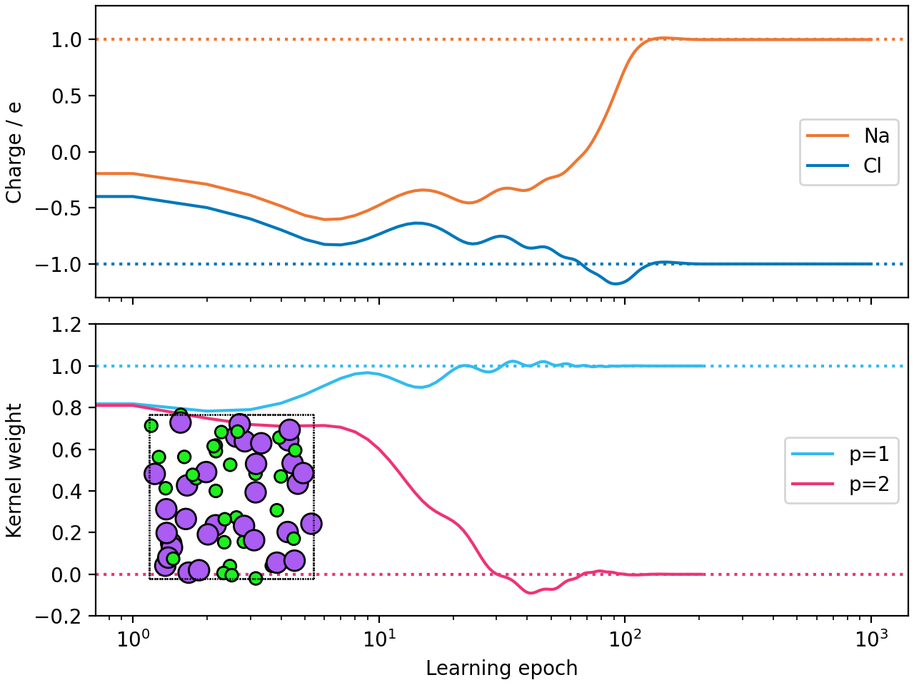
Plot results
Visualize the learning process for charges and kernel weights.
palette = [
    "#EE7733",  # Orange
    "#0077BB",  # Blue
    "#33BBEE",  # Light Blue
    "#EE3377",  # Pink
    "#CC3311",  # Red
    "#009988",  # Teal
    "#BBBBBB",  # Grey
    "#000000",  # Black
]


def plot_results(fname=None, show_snapshot=True):
    """
    Plot the learning process for charges and kernel weights.

    Args:
        fname (str): File name to save the plot. If None, the plot is not saved.
        show_snapshot (bool): Whether to show a snapshot of the atomic configuration.
    """
    fig, ax = plt.subplots(
        2,
        sharex=True,
        layout="constrained",
        dpi=200,
    )

    if show_snapshot:
        ax_in = fig.add_axes([0.12, 0.14, 0.27, 0.27])
        ase.visualize.plot.plot_atoms(atoms, ax=ax_in, radii=0.75)
        ax_in.set_axis_off()

    # Plot charge learning
    ax[0].plot(q_Na_timeseries, c=palette[0], label=r"Na")
    ax[0].plot(np.array(q_Cl_timeseries), c=palette[1], label=r"Cl")

    ax[0].set_ylim(-1.3, 1.3)
    ax[0].axhline(1, ls="dotted", c=palette[0])
    ax[0].axhline(-1, ls="dotted", c=palette[1])
    ax[0].legend()
    ax[0].set_ylabel(r"Charge / e")

    # Plot kernel weight learning
    ax[1].axhline(1, c=palette[2], ls="dotted")
    ax[1].axhline(0, c=palette[3], ls="dotted")
    weights_timeseries_array = np.array(weights_timeseries)
    ax[1].plot(weights_timeseries_array[:, 0], label="p=1", c=palette[2])
    ax[1].plot(weights_timeseries_array[:, 1], label="p=2", c=palette[3])

    ax[1].set_ylim(-0.2, 1.2)
    ax[1].legend()
    ax[1].set_ylabel("Kernel weight")

    for a in ax:
        a.set_xscale("log")

    ax[1].set_xlabel("Learning epoch")

    fig.align_labels()

    if fname is not None:
        fig.savefig(fname, transparent=True, bbox_inches="tight")

    plt.show()


# Call the plot function to visualize results
plot_results(show_snapshot=True)
Total running time of the script: (1 minutes 21.254 seconds)