Long-stride trajectories with a universal FlashMD model

Authors:

Michele Ceriotti @ceriottm

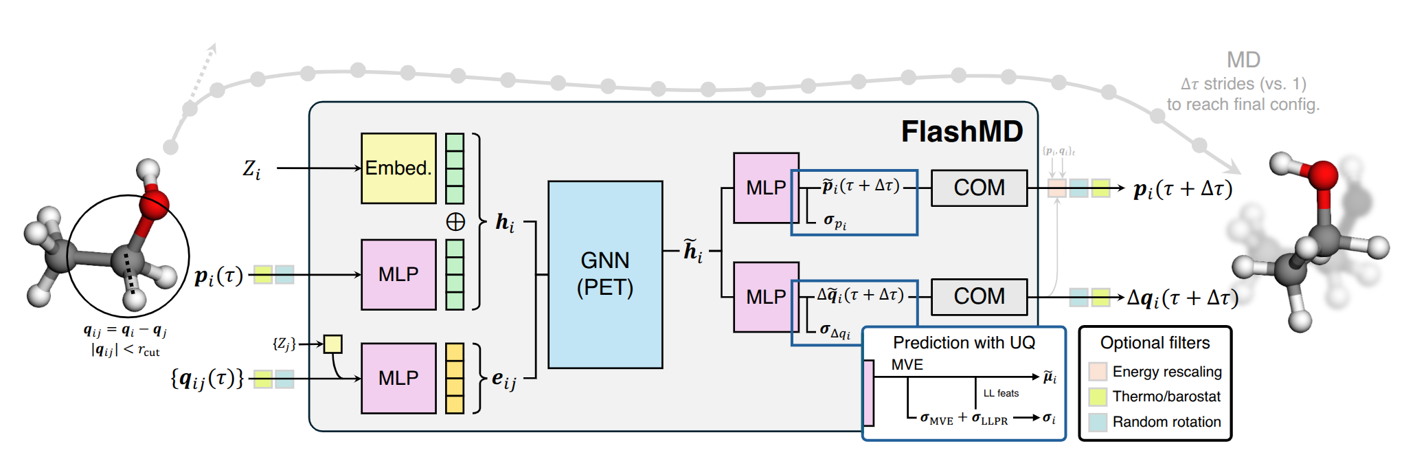
This example demonstrates how to run long-stride molecular dynamics using the universal FlashMD model. FlashMD predicts directly positions and momenta of atoms at a later time based on the current positions and momenta. It is trained on MD trajectories obtained with the PET-MAD universal potential. You can read more about the model and its limitations in this preprint.

Start by importing the required libraries. You will need the PET-MAD potential, as well as FlashMD and a recent version of i-PI.

pip install pet-mad flashmd ipi

import chemiscope
import matplotlib.image as mpimg
import matplotlib.pyplot as plt
from flashmd import get_universal_model
from flashmd.ipi import get_npt_stepper, get_nvt_stepper
from ipi.utils.parsing import read_output, read_trajectory
from ipi.utils.scripting import InteractiveSimulation
from pet_mad.calculator import PETMADCalculator

A rough schematic of the architecture of FlashMD is shown below. Each model is trained for a specific stride length, aiming to reproduce the trajectories obtained with a traditional velocity Verlet integrator.

# use matplotlib to display the image so it also display as a thumbnail
fig, ax = plt.subplots(figsize=(5728 / 300, 2598 / 300), dpi=300)
img = mpimg.imread("flashmd-scheme.png")
ax.imshow(img)
ax.axis("off")
fig.tight_layout()
plt.show()

We start by getting the FlashMD models from the flashmd package. We will also use the PET-MAD universal potential as an accompanying energy model

device = "cpu"  # change to "cuda" if you have a GPU; don't forget to change it in the
# i-PI xml input files as well!

flashmd_model_16 = get_universal_model(16)
flashmd_model_16.to(device)

flashmd_model_64 = get_universal_model(64)
flashmd_model_64.to(device)

calculator = PETMADCalculator(version="latest", device=device)
calculator._model.save("pet-mad-latest.pt")

Al(110) surface dynamics

The (110) surface of aluminum exhibits an interesting dynamical behavior well below the bulk melting temperature. This manifests itself in the spontaneous formation of surface defects, with mobile adatoms emerging at the surface.

We run a FlashMD simulation with 64 fs strides (as opposed to 1 or 2 fs) at 600 K, observing the motion of the adatom at the surface. We use the i-PI scripting API to set up the simulation and run it interactively.

The starting point is a “base” XML file that contains the setup for a traditional MD simulation in i-PI. It contains PET-MAD as the potential energy calculator (needed for the optional energy rescaling filter), and the only difference is the use of a much larger large time step than conventional MD.

with open("data/input-al110-base.xml", "r") as input_xml:
    sim = InteractiveSimulation(input_xml)

 @system: Initializing system object
 @simulation: Initializing simulation object
@ RANDOM SEED: The seed used in this calculation was 32123
 @init_file: Initializing from file data/al110.xyz. Dimension: length, units: automatic, cell_units: automatic
 @init_file: Initializing from file data/al110.xyz. Dimension: length, units: automatic, cell_units: automatic
 @init_file: Initializing from file data/al110.xyz. Dimension: length, units: automatic, cell_units: automatic
 @init_file: Initializing from file data/al110.xyz. Dimension: length, units: automatic, cell_units: automatic
 @init_file: Initializing from file data/al110.xyz. Dimension: length, units: automatic, cell_units: automatic
 @initializer: Resampling velocities at temperature 600.0 kelvin
 @system.bind: Binding the forces

To run FlashMD, we set up a custom step, using the get_nvt_stepper utility function from the flashmd.ipi module. Note the filters rescale_energy=True and random_rotation=True. The first one ensures that the total energy of the system is conserved, while the second one allows for random rotations of the system, which is useful to correct for the fact that the model is not exactly equivariant with respect to rotations.

sim.set_motion_step(
    get_nvt_stepper(
        sim, flashmd_model_64, device, rescale_energy=True, random_rotation=True
    )
)

# run for a few steps - this is a large box, and is rather slow on CPU
sim.run(20)

@simulation.run: Average timings at MD step       0. t/step: 6.35806e+00

The trajectory is stable, and one can check that the mean fluctuations of the adatom are qualitatively correct, by comparing with a (much slower) PET-MAD simulation.

data, info = read_output("al110-nvt-flashmd.out")
trj = read_trajectory("al110-nvt-flashmd.pos_0.extxyz")

chemiscope.show(
    frames=trj,
    properties={
        "time": data["time"],
        "potential": data["potential"],
        "temperature": data["temperature"],
    },
    mode="default",
    settings=chemiscope.quick_settings(
        map_settings={
            "x": {"property": "time", "scale": "linear"},
            "y": {"property": "potential", "scale": "linear"},
        },
        structure_settings={
            "unitCell": True,
        },
        trajectory=True,
    ),
)

×

Solvated alanine dipeptide

As a second example, we run a constant-pressure simulation of explicitly solvated alanine dipeptide, using the FlashMD universal model with 16 fs time steps (as opposed to 0.5 fs). The setup is very similar to the previous example, but we use an input template that contains a NpT setup, and use the get_npt_stepper utility function to set up a stepper that combine the FlashMD velocity-Verlet step with cell updates.

with open("data/input-ala2-base.xml", "r") as input_xml:
    sim = InteractiveSimulation(input_xml)

sim.set_motion_step(
    get_npt_stepper(
        sim, flashmd_model_16, device, rescale_energy=True, random_rotation=True
    )
)
sim.run(10)  # only run 10 steps, again, pretty slow on CPU

 @system: Initializing system object
 @simulation: Initializing simulation object
@ RANDOM SEED: The seed used in this calculation was 32123
 @init_file: Initializing from file data/ala2.xyz. Dimension: length, units: automatic, cell_units: automatic
 @init_file: Initializing from file data/ala2.xyz. Dimension: length, units: automatic, cell_units: automatic
 @init_file: Initializing from file data/ala2.xyz. Dimension: length, units: automatic, cell_units: automatic
 @init_file: Initializing from file data/ala2.xyz. Dimension: length, units: automatic, cell_units: automatic
 @init_file: Initializing from file data/ala2.xyz. Dimension: length, units: automatic, cell_units: automatic
 @initializer: Resampling velocities at temperature 450.0 kelvin
 @system.bind: Binding the forces
 @simulation.run: Average timings at MD step       0. t/step: 1.48012e+01
 @open_backup: Backup performed: RESTART -> #RESTART#0#

The cell fluctuates around the equilibrium volume, in a way that is consistent with the correct NpT ensemble. The trajectory is stable and the alanine molecule explores the different conformations (obviously when running for a reasonably long time).

data, info = read_output("ala2-npt-flashmd.out")
trj = read_trajectory("ala2-npt-flashmd.pos_0.extxyz")

chemiscope.show(
    frames=trj,
    properties={
        "time": data["time"],
        "volume": data["volume"],
        "potential": data["potential"],
        "pressure": data["pressure_md"],
        "temperature": data["temperature"],
    },
    mode="default",
    settings=chemiscope.quick_settings(
        map_settings={
            "x": {"property": "time", "scale": "linear"},
            "y": {"property": "volume", "scale": "linear"},
        },
        structure_settings={
            "unitCell": True,
        },
        trajectory=True,
    ),
)

×