Atomistic Water Model for Molecular Dynamics

Authors:

Philip Loche @PicoCentauri, Marcel Langer @sirmarcel and Michele Ceriotti @ceriottm

In this example, we demonstrate how to construct a metatomic model for flexible three and four-point water model, with parameters optimized for use together with quantum-nuclear-effects-aware path integral simulations (cf. Habershon et al., JCP (2009)). The model also demonstrates the use of torch-pme, a Torch library for long-range interactions, and uses the resulting model to perform demonstrative molecular dynamics simulations.

# sphinx_gallery_thumbnail_number = 3

import subprocess
from typing import Dict, List, Optional, Tuple

import ase.io

# Simulation and visualization tools
import chemiscope
import matplotlib.pyplot as plt

# Model wrapping and execution tools
import numpy as np
import torch

# Core atomistic libraries
import torchpme
from ase.optimize import LBFGS
from ipi.utils.parsing import read_output, read_trajectory
from ipi.utils.scripting import (
    InteractiveSimulation,
    forcefield_xml,
    motion_nvt_xml,
    simulation_xml,
)
from metatensor.torch import Labels, TensorBlock, TensorMap
from metatomic.torch import (
    AtomisticModel,
    ModelCapabilities,
    ModelEvaluationOptions,
    ModelMetadata,
    ModelOutput,
    NeighborListOptions,
    System,
    load_atomistic_model,
)

# Integration with ASE calculator for metatomic models
from metatomic.torch.ase_calculator import MetatomicCalculator
from vesin.torch.metatensor import NeighborList

The q-TIP4P/F Model

The q-TIP4P/F model uses simple (quasi)-harmonic terms to describe intra-molecular flexibility - with the use of a quartic term being a specific feature used to describe the covalent bond softening for a H-bonded molecule - a Lennard-Jones term describing dispersion and repulsion between O atoms, and an electrostatic potential between partial charges on the H atoms and the oxygen electron density. For a four-point model, the oxygen charge is slightly displaced from the oxygen’s position, improving properties like the dielectric constant. The fourth point, referred to as M, is implicitly derived from the other atoms of each water molecule.

Intra-molecular interactions

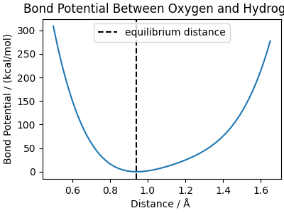
The molecular bond potential is usually defined as a harmonic potential of the form

\[V_\mathrm{bond}(r) = \frac{k_\mathrm{bond}}{2} (r - r_0)^2\]

Here, \(k_\mathrm{bond}\) is the force constant and \(r_0\) is the equilibrium distance. Bonded terms like this require defining a topology, i.e. a list of pairs of atoms that are actually bonded to each other.

q-TIP4P/F doesn’t use a harmonic potential but a quartic approximation of a Morse potential, that allows describing the anharmonicity of the O-H covalent bond, and how the mean distance changes due to zero-point fluctuations and/or hydrogen bonding.

\[V_\mathrm{bond}(r) = \frac{k_r}{2} [(r-r_0)^2-\alpha_r (r-r_0)^3 + \frac{7}{12}\alpha_r^2(r-r_0)^4]\]

Note

The harmonic coefficient is related to the coefficients in the original paper by \(k_r=2 D_r \alpha_r^2\).

def bond_energy(
    distances: torch.Tensor,
    coefficient_k: torch.Tensor,
    coefficient_alpha: torch.Tensor,
    coefficient_r0: torch.Tensor,
) -> torch.Tensor:
    """Harmonic potential for bond terms."""
    dr = distances - coefficient_r0
    alpha_dr = dr * coefficient_alpha

    return 0.5 * coefficient_k * dr**2 * (1 - alpha_dr + alpha_dr**2 * 7 / 12)

The parameters reproduce the form of a Morse potential close to the minimum, but avoids the dissociation of the bond, due to the truncation to the quartic term. These are the parameters used for q-TIP4P/F

OH_kr = 116.09 * 2 * 2.287**2  # kcal/mol/Å**2
OH_r0 = 0.9419  # Å
OH_alpha = 2.287  # 1/Å

bond_distances = np.linspace(0.5, 1.65, 200)
bond_potential = bond_energy(
    distances=bond_distances,
    coefficient_k=OH_kr,
    coefficient_alpha=OH_alpha,
    coefficient_r0=OH_r0,
)

fig, ax = plt.subplots(1, 1, figsize=(4, 3), constrained_layout=True)
ax.set_title("Bond Potential Between Oxygen and Hydrogen")

ax.plot(bond_distances, bond_potential)
ax.axvline(OH_r0, label="equilibrium distance", color="black", linestyle="--")

ax.set_xlabel("Distance / Å ")
ax.set_ylabel("Bond Potential / (kcal/mol)")

ax.legend()
fig.show()

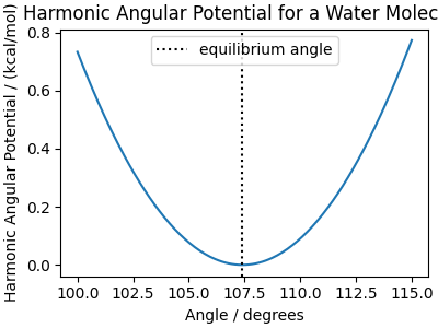
The harmonic angle potential describe the bending of the HOH angle, and is usually modeled as a (curvilinear) harmonic term, defined based on the angle

\[V_\mathrm{angle}(\theta) = \frac{k_\mathrm{angle}}{2} (\theta - \theta_0)^2\]

where \(k_\mathrm{angle}\) is the force constant and \(\theta_0\) is the equilibrium angle between the three atoms.

def bend_energy(
    angles: torch.Tensor, coefficient: torch.Tensor, equilibrium_angle: torch.Tensor
):
    """Harmonic potential for angular terms."""
    return 0.5 * coefficient * (angles - equilibrium_angle) ** 2

We use the following parameters:

HOH_angle_coefficient = 87.85  # kcal/mol/rad^2
HOH_equilibrium_angle = 107.4 * torch.pi / 180  # radians

We can plot the bend energy as a function of the angle that is, unsurprisingly, parabolic around the equilibrium angle

angle_distances = np.linspace(100, 115, 200)
angle_potential = bend_energy(
    angles=angle_distances * torch.pi / 180,
    coefficient=HOH_angle_coefficient,
    equilibrium_angle=HOH_equilibrium_angle,
)

fig, ax = plt.subplots(1, 1, figsize=(4, 3), constrained_layout=True)
ax.set_title("Harmonic Angular Potential for a Water Molecule")

ax.plot(angle_distances, angle_potential)
ax.axvline(
    HOH_equilibrium_angle * 180 / torch.pi,
    label="equilibrium angle",
    color="black",
    linestyle=":",
)

ax.set_xlabel("Angle / degrees")
ax.set_ylabel("Harmonic Angular Potential / (kcal/mol)")

ax.legend()
fig.show()

Lennard-Jones Potential

The Lennard-Jones (LJ) potential describes the interaction between a pair of neutral atoms or molecules, balancing dispersion forces at longer ranges and repulsive forces at shorter ranges. The LJ potential is defined as:

\[V_\mathrm{LJ}(r) = 4 \epsilon \left[ \left( \frac{\sigma}{r} \right)^{12} - \left( \frac{\sigma}{r} \right)^6 \right]\]

where \(\epsilon\) is the depth of the potential well and \(\sigma\) the distance at which the potential is zero. For water there is usually only an oxygen-oxygen Lennard-Jones potential.

We implement the Lennard-Jones potential as a function that takes distances, along with the parameters sigma, epsilon, and cutoff that indicates the distance at which the interaction is assumed to be zero. To ensure that there is no discontinuity an offset is included to shift the curve so it is zero at the cutoff distance.

def lennard_jones_pair(
    distances: torch.Tensor,
    sigma: torch.Tensor,
    epsilon: torch.Tensor,
    cutoff: torch.Tensor,
):
    """Shifted Lennard-Jones potential for pair terms."""
    c6 = (sigma / distances) ** 6
    c12 = c6**2
    lj = 4 * epsilon * (c12 - c6)

    sigma_cutoff_6 = (sigma / cutoff) ** 6
    offset = 4 * epsilon * sigma_cutoff_6 * (sigma_cutoff_6 - 1)

    return lj - offset

We plot this potential to visualize its behavior, using q-TIP4P/F parameters. To highlight the offset, we use a cutoff of 5 Å instead of the usual 7 Å.

O_sigma = 3.1589  # Å
O_epsilon = 0.1852  # kcal/mol
cutoff = 5.0  # Å <- cut short, to highlight offset

lj_distances = np.linspace(3, cutoff, 200)

lj_potential = lennard_jones_pair(
    distances=lj_distances, sigma=O_sigma, epsilon=O_epsilon, cutoff=cutoff
)

fig, ax = plt.subplots(1, 1, figsize=(4, 3), constrained_layout=True)
ax.set_title("Lennard-Jones Potential Between Two Oxygen Atoms")
ax.axhline(0, color="black", linestyle="--")
ax.axhline(-O_epsilon, color="red", linestyle=":", label="Oxygen ε")
ax.axvline(O_sigma, color="black", linestyle=":", label="Oxygen σ")
ax.plot(lj_distances, lj_potential)
ax.set_xlabel("Distance / Å")
ax.set_ylabel("Lennard-Jones Potential / (kcal/mol)")
ax.legend()
fig.show()

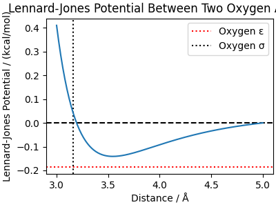
Due to our reduced cutoff the minimum of the blue line does not touch the red horizontal line.

Electrostatic Potential

The long-ranged nature of electrostatic interactions makes computing them in simulations non-trivial. For periodic systems the Coulomb energy is given by:

\[V_\mathrm{Coulomb} = \frac{1}{2} \sum_{i,j} \sideset{}{'}\sum_{\boldsymbol n \in \mathcal{Z}} \frac{1}{4\pi\epsilon_0} \frac{q_i q_j}{\left|\boldsymbol r_{ij} + \boldsymbol{n L}\right|}\]

The sum over \(\boldsymbol n\) takes into account the periodic images of the charges and the prime indicates that in the case \(i=j\) the term \(n=0\) must be omitted. Further \(\boldsymbol r_{ij} = \boldsymbol r_i - \boldsymbol r_j\) and \(\boldsymbol L\) is the length of the (cubic)simulation box.

Since this sum is conditionally convergent it isn’t computable using a direct sum. Instead the Ewald summation, published in 1921, remains a foundational method that effectively defines how to compute the energy and forces of such systems. To further speed the methods, mesh based algorithm suing fast Fourier transformation have been developed, such as the Particle-Particle Particle-Mesh (P3M) algorithm. For further details we refer to a paper by Deserno and Holm.

We use a Torch implementation of the P3M method within the torch-pme package. The core class we use is the torchpme.P3MCalculator class - you can read more and see specific examples in the torchpme documentation As a demonstration we use two charges in a cubic cell, computing the electrostatic energy as a function of distance

O_charge = -0.84
coulomb_distances = torch.linspace(0.5, 9.0, 50)
cell = torch.eye(3) * 10.0

We also use the parameter-tuning functionality of torchpme, to provide efficient evaluation at the desired level of accuracy. This is achieved calling torchpme.tuning.tune_p3m() on a template of the target structure

charges = torch.tensor([O_charge, -O_charge]).unsqueeze(-1)
positions_coul = torch.tensor([[0.0, 0.0, 0.0], [4.0, 0.0, 0.0]])
neighbor_indices = torch.tensor([[0, 1]])
neighbor_distances = torch.tensor([4.0])

p3m_smearing, p3m_parameters, _ = torchpme.tuning.tune_p3m(
    charges,
    cell,
    positions_coul,
    cutoff,
    neighbor_indices,
    neighbor_distances,
    accuracy=1e-4,
)
p3m_prefactor = torchpme.prefactors.kcalmol_A

The hydrogen charge is derived from the oxygen charge as \(q_H = -q_O/2\). The smearing and mesh_spacing parameters are the central parameters for P3M and are crucial to ensure the correct energy calculation. We now compute the electrostatic energy between two point charges using the P3M algorithm.

p3m_calculator = torchpme.P3MCalculator(
    potential=torchpme.CoulombPotential(p3m_smearing),
    **p3m_parameters,
    prefactor=p3m_prefactor,
)

For the inference, we need a neighbor list and distances which we compute “manually”. Typically, the neighbors are provided by the simulation engine.

neighbor_indices = torch.tensor([[0, 1]])

potential = torch.zeros_like(coulomb_distances)

for i_dist, dist in enumerate(coulomb_distances):
    positions_coul = torch.tensor([[0.0, 0.0, 0.0], [dist, 0.0, 0.0]])
    charges = torch.tensor([O_charge, -O_charge]).unsqueeze(-1)

    neighbor_distances = torch.tensor([dist])

    potential[i_dist] = p3m_calculator.forward(
        positions=positions_coul,
        cell=cell,
        charges=charges,
        neighbor_indices=neighbor_indices,
        neighbor_distances=neighbor_distances,
    )[0]

We plot the electrostatic potential between two point charges.

fig, ax = plt.subplots(1, 1, figsize=(4, 3), constrained_layout=True)

ax.set_title("Electrostatic Potential Between Two Point Charges")
ax.plot(coulomb_distances, potential)

ax.set_xlabel("Distance / Å")
ax.set_ylabel("Electrostatic Potential / (kcal/mol)")

fig.show()

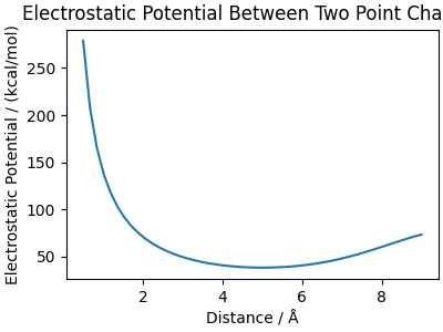
The potential shape may appear unusual due to computations within a periodic box. For small distances, the potential behaves like \(1/r\), but it increases again as charges approach across periodic boundaries.

Note

In most water models, Coulomb interactions within each molecule are excluded, as intramolecular energies are already parametrized by the bond and angle interactions. Therefore, in our model defined below we first compute the electrostatic energy of all atoms and then subtract interactions between bonded atoms.

Implementation as a TIP4P/f torch module

In order to implement a Q-TIP4P/f potential in practice, we first build a class that follows the interface of a metatomic model. This requires defining the atomic structure in terms of a metatomic.torch.System object - a simple container for positions, cell, and atomic types, that can also be enriched with one or more metatomic.torchist objects holding neighbor distance information. This is usually provided by the code used to perform a simulation, but can be also computed explicitly using ase or vesin, as we do here.

For running our simulation we use a small waterbox containing 32 water molecules.

atoms = ase.io.read("data/water_32.xyz")

chemiscope.show(
    [atoms],
    mode="structure",
    settings=chemiscope.quick_settings(structure_settings={"unitCell": True}),
)

×

We transform the ase Atoms object into a metatomic system and define the options for the neighbor list.

system = System(
    types=torch.from_numpy(atoms.get_atomic_numbers()),
    positions=torch.from_numpy(atoms.positions),
    cell=torch.from_numpy(atoms.cell.array),
    pbc=torch.from_numpy(atoms.pbc),
)

nlo = NeighborListOptions(cutoff=7.0, full_list=False, strict=False)
calculator = NeighborList(nlo, length_unit="Angstrom")
neighbors = calculator.compute(system)
system.add_neighbor_list(nlo, neighbors)

Neighbor lists are stored within metatensor as metatensor.TensorBlock objects, if you’re curious

neighbors

TensorBlock
    samples (6001): ['first_atom', 'second_atom', 'cell_shift_a', 'cell_shift_b', 'cell_shift_c']
    components (3): ['xyz']
    properties (1): ['distance']
    gradients: None

Helper functions for molecular geometry

In order to compute the different terms in the Q-TIP4P/f potential, we need to extract some information on the geometry of the water molecule. To keep the model class clean, we define a helper functions that do two things.

First, it computes O-H covalent bond lengths and angle. We use heuristics to identify the covalent bonds as the shortest O-H distances in a simulation. This is necessary when using the model with an external code, that might re-order atoms internally (as is e.g. the case for LAMMPS). The heuristics here may fail in case molecules get too close together, or at very high temperature.

Second, it computes the position of the virtual “M sites”, the position of the O charge in a TIP4P-like model. We also need distances to compute range-separated electrostatics, which we obtain manipulating the neighbor list that is pre-attached to the system. Thanks to the fact we rely on torch autodifferentiation mechanism, the forces acting on the virtual sites will be automatically split between O and H atoms, in a way that is consistent with the definition.

Forces acting on the M sites will be automatically split between O and H atoms, in a way that is consistent with the definition.

def get_molecular_geometry(
    system: System,
    nlo: NeighborListOptions,
    m_gamma: torch.Tensor,
    m_charge: torch.Tensor,
) -> Tuple[torch.Tensor, torch.Tensor, System, torch.Tensor, torch.Tensor]:
    """Compute bond distances, angles and charge site positions for each molecules."""
    neighbors = system.get_neighbor_list(nlo)
    species = system.types

    # get neighbor idx and vectors as torch tensors
    neigh_ij = neighbors.samples.view(["first_atom", "second_atom"]).values
    neigh_dij = neighbors.values.squeeze()

    # get all OH distances and their sorting order
    oh_mask = species[neigh_ij[:, 0]] != species[neigh_ij[:, 1]]
    oh_ij = neigh_ij[oh_mask]
    oh_dij = neigh_dij[oh_mask]
    oh_dist = torch.linalg.vector_norm(oh_dij, dim=1).squeeze()
    oh_sort = torch.argsort(oh_dist)

    # gets the oxygen indices in the bonds, sorted by distance
    oh_oidx = torch.where(species[oh_ij[:, 0]] == 8, oh_ij[:, 0], oh_ij[:, 1])[oh_sort]
    # makes sure we always consider bonds in the O->H direction
    oh_dij = oh_dij * torch.where(species[oh_ij[:, 0]] == 8, 1.0, -1.0).reshape(-1, 1)

    # we assume that the first n_oxygen*2 bonds cover all water molecules.
    # if not we throw an error
    o_idx = torch.nonzero(species == 8).squeeze()
    n_oh = len(o_idx) * 2
    oh_oidx_sort = torch.argsort(oh_oidx[:n_oh])

    oh_dij_oidx = oh_oidx[oh_oidx_sort]  # indices of the O atoms for each dOH
    # if each O index appears twice, this should be a vector of zeros
    twoo_chk = oh_dij_oidx[::2] - oh_dij_oidx[1::2]
    if (twoo_chk != 0).any():
        raise RuntimeError("Cannot assign OH bonds to water molecules univocally.")

    # finally, we compute O->H1 and O->H2 for each water molecule
    oh_dij_sort = oh_dij[oh_sort[:n_oh]][oh_oidx_sort]
    doh_1 = oh_dij_sort[::2]
    doh_2 = oh_dij_sort[1::2]

    oh_dist = torch.concatenate(
        [
            torch.linalg.vector_norm(doh_1, dim=1),
            torch.linalg.vector_norm(doh_2, dim=1),
        ]
    )

    if oh_dist.max() > 2.0:
        raise ValueError(
            "Unphysical O-H bond length. Check that the molecules are entire, and "
            "atoms are listed in the expected OHH order."
        )

    hoh_angles = torch.arccos(
        torch.sum(doh_1 * doh_2, dim=1)
        / (oh_dist[: len(doh_1)] * oh_dist[len(doh_2) :])
    )

    # now we use this information to build the M sites
    # we first put the O->H vectors in the same order as the
    # positions. This allows us to manipulate all atoms at once later
    oh1_vecs = torch.zeros_like(system.positions)
    oh1_vecs[oh_dij_oidx[::2]] = doh_1
    oh2_vecs = torch.zeros_like(system.positions)
    oh2_vecs[oh_dij_oidx[1::2]] = doh_2

    # we compute the vectors O->M displacing the O to the M sites
    om_displacements = (1 - m_gamma) * 0.5 * (oh1_vecs + oh2_vecs)

    # creates a new System with the m-sites
    m_system = System(
        types=system.types,
        positions=system.positions + om_displacements,
        cell=system.cell,
        pbc=system.pbc,
    )

    # adjust neighbor lists to point at the m sites rather than O atoms. this assumes
    # this won't have atoms cross the cutoff, which is of course only approximately
    # true, so one should use a slighlty larger-than-usual cutoff nb - this is reshaped
    # to match the values in a NL tensorblock
    nl = system.get_neighbor_list(nlo)
    i_idx = nl.samples.view(["first_atom"]).values.flatten()
    j_idx = nl.samples.view(["second_atom"]).values.flatten()
    m_nl = TensorBlock(
        nl.values
        + (om_displacements[j_idx] - om_displacements[i_idx]).reshape(-1, 3, 1),
        nl.samples,
        nl.components,
        nl.properties,
    )
    m_system.add_neighbor_list(nlo, m_nl)

    # set charges of all atoms
    charges = (
        torch.where(species == 8, -m_charge, 0.5 * m_charge)
        .reshape(-1, 1)
        .to(dtype=system.positions.dtype, device=system.positions.device)
    )

    # Create metadata for the charges TensorBlock
    samples = Labels(
        "atom", torch.arange(len(system), device=charges.device).reshape(-1, 1)
    )
    properties = Labels(
        "charge", torch.zeros(1, 1, device=charges.device, dtype=torch.int32)
    )
    data = TensorBlock(
        values=charges, samples=samples, components=[], properties=properties
    )

    tensor = TensorMap(
        keys=Labels("_", torch.zeros(1, 1, device=charges.device, dtype=torch.int32)),
        blocks=[data],
    )

    m_system.add_data(name="charges", tensor=tensor)

    # intra-molecular distances with M sites (for self-energy removal)
    hh_dist = torch.sqrt(((doh_1 - doh_2) ** 2).sum(dim=1))
    dmh_1 = doh_1 - om_displacements[oh_dij_oidx[::2]]
    dmh_2 = doh_2 - om_displacements[oh_dij_oidx[1::2]]
    mh_dist = torch.concatenate(
        [
            torch.linalg.vector_norm(dmh_1, dim=1),
            torch.linalg.vector_norm(dmh_2, dim=1),
        ]
    )

    return oh_dist, hoh_angles, m_system, mh_dist, hh_dist

Defining the model

Armed with these functions, the definitions of bonded and LJ potentials, and the torchpme.P3MCalculator class, we can define with relatively small effort the actual model. We do not hard-code the specific parameters of the Q-TIP4P/f potential (so that in principle this class can be used for classical TIP4P, and - by setting m_gamma to one - a three-point water model).

A few points worth noting: (1) As discussed above we define a bare Coulomb potential (that pretty much computes \(1/r\)) which we need to subtract the molecular “self electrostatic interaction”; (2) units are expected to be Å for distances, kcal/mol for energies, and radians for angles; (3) model parameters are registered as buffers; (4) P3M parameters can also be given, in the format returned by torchpme.tuning.tune_p3m().

The forward call is a relatively straightforward combination of all the helper functions defined further up in this file, and should be relatively easy to follow.

class WaterModel(torch.nn.Module):
    def __init__(
        self,
        cutoff: float,
        lj_sigma: float,
        lj_epsilon: float,
        m_gamma: float,
        m_charge: float,
        oh_bond_eq: float,
        oh_bond_k: float,
        oh_bond_alpha: float,
        hoh_angle_eq: float,
        hoh_angle_k: float,
        p3m_options: Optional[dict] = None,
    ):
        super().__init__()

        if p3m_options is None:
            # should give a ~1e-4 relative accuracy on forces
            p3m_options = (1.4, {"interpolation_nodes": 5, "mesh_spacing": 1.33}, 0)

        p3m_smearing, p3m_parameters, _ = p3m_options

        self.p3m_calculator = torchpme.metatensor.P3MCalculator(
            potential=torchpme.CoulombPotential(p3m_smearing),
            **p3m_parameters,
            prefactor=torchpme.prefactors.kcalmol_A,  # consistent units
        )

        self.coulomb = torchpme.CoulombPotential()

        # We use a half neighborlist and allow to have pairs farther than cutoff
        # (`strict=False`) since this is not problematic for PME and may speed up the
        # computation of the neigbors.
        self.nlo = NeighborListOptions(cutoff=cutoff, full_list=False, strict=False)

        self.register_buffer("cutoff", torch.tensor(cutoff))
        self.register_buffer("lj_sigma", torch.tensor(lj_sigma))
        self.register_buffer("lj_epsilon", torch.tensor(lj_epsilon))
        self.register_buffer("m_gamma", torch.tensor(m_gamma))
        self.register_buffer("m_charge", torch.tensor(m_charge))
        self.register_buffer("oh_bond_eq", torch.tensor(oh_bond_eq))
        self.register_buffer("oh_bond_k", torch.tensor(oh_bond_k))
        self.register_buffer("oh_bond_alpha", torch.tensor(oh_bond_alpha))
        self.register_buffer("hoh_angle_eq", torch.tensor(hoh_angle_eq))
        self.register_buffer("hoh_angle_k", torch.tensor(hoh_angle_k))

    def requested_neighbor_lists(self):
        """Returns the list of neighbor list options that are needed."""
        return [self.nlo]

    def _setup_systems(
        self,
        systems: list[System],
        selected_atoms: Optional[Labels] = None,
    ) -> tuple[System, TensorBlock]:
        if len(systems) > 1:
            raise ValueError(f"only one system supported, got {len(systems)}")

        system_i = 0
        system = systems[system_i]

        # select only real atoms and discard ghosts
        # (this is to work in codes like LAMMPS that provide a neighbor
        # list that also includes "domain decomposition" neigbhbors)
        if selected_atoms is not None:
            current_system_mask = selected_atoms.column("system") == system_i
            current_atoms = selected_atoms.column("atom")
            current_atoms = current_atoms[current_system_mask].to(torch.long)

            types = system.types[current_atoms]
            positions = system.positions[current_atoms]
            system_clean = System(types, positions, system.cell, system.pbc)
            for nlo in system.known_neighbor_lists():
                system_clean.add_neighbor_list(nlo, system.get_neighbor_list(nlo))
        else:
            system_clean = system
        return system_clean, system.get_neighbor_list(self.nlo)

    def forward(
        self,
        systems: List[System],  # noqa
        outputs: Dict[str, ModelOutput],  # noqa
        selected_atoms: Optional[Labels] = None,
    ) -> Dict[str, TensorMap]:  # noqa

        if list(outputs.keys()) != ["energy"]:
            raise ValueError(
                f"`outputs` keys ({', '.join(outputs.keys())}) contain unsupported "
                "keys. Only 'energy' is supported."
            )

        if outputs["energy"].per_atom:
            raise NotImplementedError("per-atom energies are not supported.")

        system, neighbors = self._setup_systems(systems, selected_atoms)

        # compute non-bonded LJ energy
        neighbor_indices = neighbors.samples.view(["first_atom", "second_atom"]).values
        species = system.types
        oo_mask = (species[neighbor_indices[:, 0]] == 8) & (
            species[neighbor_indices[:, 1]] == 8
        )
        oo_distances = torch.linalg.vector_norm(neighbors.values[oo_mask], dim=1)
        energy_lj = lennard_jones_pair(
            oo_distances, self.lj_sigma, self.lj_epsilon, self.cutoff
        ).sum()

        d_oh, a_hoh, m_system, mh_dist, hh_dist = get_molecular_geometry(
            system, self.nlo, self.m_gamma, self.m_charge
        )

        # intra-molecular energetics
        e_bond = bond_energy(
            d_oh, self.oh_bond_k, self.oh_bond_alpha, self.oh_bond_eq
        ).sum()
        e_bend = bend_energy(a_hoh, self.hoh_angle_k, self.hoh_angle_eq).sum()

        # now this is the long-range part - computed over the M-site system
        # m_system, mh_dist, hh_dist = get_msites(system, self.m_gamma, self.m_charge)
        m_neighbors = m_system.get_neighbor_list(self.nlo)

        potentials = self.p3m_calculator(m_system, m_neighbors).block(0).values
        charges = m_system.get_data("charges").block().values
        energy_coulomb = (potentials * charges).sum()

        # this is the intra-molecular Coulomb interactions, that must be removed
        # to avoid double-counting
        energy_self = (
            (
                self.coulomb.from_dist(mh_dist).sum() * (-self.m_charge)
                + self.coulomb.from_dist(hh_dist).sum() * 0.5 * self.m_charge
            )
            * 0.5
            * self.m_charge
            * torchpme.prefactors.kcalmol_A
        )

        # combines all energy terms
        energy_tot = e_bond + e_bend + energy_lj + energy_coulomb - energy_self

        # Rename property label to follow metatensor's convention for an atomistic model
        samples = Labels(
            ["system"],
            torch.arange(len(systems), device=energy_tot.device).reshape(-1, 1),
        )
        properties = Labels(["energy"], torch.tensor([[0]], device=energy_tot.device))

        block = TensorBlock(
            values=torch.sum(energy_tot).reshape(-1, 1),
            samples=samples,
            components=torch.jit.annotate(List[Labels], []),
            properties=properties,
        )
        return {
            "energy": TensorMap(
                Labels("_", torch.tensor([[0]], device=energy_tot.device)), [block]
            ),
        }

All this class does is take a System and return its energy (as a metatensor.TensorMap`).

qtip4pf_parameters = dict(
    cutoff=7.0,
    lj_sigma=3.1589,
    lj_epsilon=0.1852,
    m_gamma=0.73612,
    m_charge=1.1128,
    oh_bond_eq=0.9419,
    oh_bond_k=2 * 116.09 * 2.287**2,
    oh_bond_alpha=2.287,
    hoh_angle_eq=107.4 * torch.pi / 180,
    hoh_angle_k=87.85,
)
qtip4pf_model = WaterModel(
    **qtip4pf_parameters
    #   uncomment to override default options
    #    p3m_options = (1.4, {"interpolation_nodes": 5, "mesh_spacing": 1.33}, 0)
)

We re-initilize the system to ask for gradients

system = System(
    types=torch.from_numpy(atoms.get_atomic_numbers()),
    positions=torch.from_numpy(atoms.positions).requires_grad_(),
    cell=torch.from_numpy(atoms.cell.array).requires_grad_(),
    pbc=torch.from_numpy(atoms.pbc),
)
system.add_neighbor_list(nlo, calculator.compute(system))

energy_unit = "kcal/mol"
length_unit = "angstrom"

outputs = {"energy": ModelOutput(quantity="energy", unit=energy_unit, per_atom=False)}

nrg = qtip4pf_model.forward([system], outputs)
nrg["energy"].block(0).values.backward()

print(
    f"""
Energy is {nrg["energy"].block(0).values[0].item()} kcal/mol

The forces on the first molecule (in kcal/mol/Å) are
{system.positions.grad[:3]}

The stress is
{system.cell.grad}
"""
)

/home/runner/work/atomistic-cookbook/atomistic-cookbook/.nox/water-model/lib/python3.12/site-packages/torchpme/metatensor/calculator.py:95: UserWarning: custom data 'charges' is experimental, please contact metatensor's developers to add this data as a member of the `System` class (Triggered internally at /project/metatomic-torch/src/system.cpp:866.)
  charge_tensor = system.get_data("charges")

Energy is -274.07545584268337 kcal/mol

The forces on the first molecule (in kcal/mol/Å) are
tensor([[-22.5891,  -4.0345,  16.9057],
        [ 10.1369,   0.0815,  -0.2837],
        [  1.1909,   9.2458,  -7.3839]], dtype=torch.float64)

The stress is
tensor([[ -1.1619,  15.5917, -14.0268],
        [ 18.7409,   5.3058, -16.6880],
        [-31.6888,  -8.1921, -42.9294]], dtype=torch.float64)

Build and save an AtomisticModel

This model can be wrapped into a metatomic.torch.AtomisticModel class, that provides useful helpers to specify the capabilities of the model, and to save it as a torchscript module.

Model options include a definition of its units, and a description of the quantities it can compute.

Note

We neeed to specify that the model has infinite interaction range because of the presence of a long-range term that means one cannot assume that forces decay to zero beyond the cutoff.

options = ModelEvaluationOptions(
    length_unit=length_unit, outputs=outputs, selected_atoms=None
)

model_capabilities = ModelCapabilities(
    outputs=outputs,
    atomic_types=[1, 8],
    interaction_range=torch.inf,
    length_unit=length_unit,
    supported_devices=["cuda", "cpu"],
    dtype="float32",
)

atomistic_model = AtomisticModel(
    qtip4pf_model.eval(), ModelMetadata(), model_capabilities
)

atomistic_model.save("qtip4pf-mta.pt")

Other water models

The WaterModel class is flexible enough that one can also implement (and export) other 4-point models, or even 3-point models if one sets the m_gamma parameter to one. For instance, we can implement the (classical) SPC/Fw model (Wu et al., JCP (2006))

spcf_parameters = dict(
    cutoff=7.0,
    lj_sigma=3.16549,
    lj_epsilon=0.155425,
    m_gamma=1.0,
    m_charge=0.82,
    oh_bond_eq=1.012,
    oh_bond_k=1059.162,
    oh_bond_alpha=0.0,
    hoh_angle_eq=113.24 * torch.pi / 180,
    hoh_angle_k=75.90,
)
spcf_model = WaterModel(**spcf_parameters)

atomistic_model = AtomisticModel(spcf_model.eval(), ModelMetadata(), model_capabilities)

atomistic_model.save("spcfw-mta.pt")

Using the Q-TIP4P/f model

The torchscript model can be reused with any simulation software compatible with the metatomic API. Here we give a couple of examples, designed to demonstrate the usage more than to provide realistic use cases.

Geometry optimization with ase

We begin with an example based on an ase-compatible calculator. To this end, metatomic provides a compatible metatomic.torch.MetatomicCalculator wrapper to a model. Note how the metadata associated with the model are used to convert energy into the units expected by ase (eV and Å).

atomistic_model = load_atomistic_model("qtip4pf-mta.pt")
mta_calculator = MetatomicCalculator(atomistic_model)

atoms.calc = mta_calculator
nrg = atoms.get_potential_energy()

print(
    f"""
Energy is {nrg} eV, corresponding to {nrg*23.060548} kcal/mol
"""
)

the model suggested to use CUDA devices before CPU, but we are unable to find it

Energy is -11.8850679397583 eV, corresponding to -274.0761797080574 kcal/mol

We then use one of the built-in ase functions to run the structural relaxation. The relaxation is split into short segments just to be able to visualize the trajectory.

fmax is the threshold on the maximum force component and the optimization will stop when the threshold is reached

opt_trj = []
opt_nrg = []

for _ in range(10):
    opt_trj.append(atoms.copy())
    opt_nrg.append(atoms.get_potential_energy())
    opt = LBFGS(atoms, restart="lbfgs_restart.json")
    opt.run(fmax=0.001, steps=5)

opt.run(fmax=0.001, steps=10)
nrg_final = atoms.get_potential_energy()

       Step     Time          Energy          fmax
LBFGS:    0 14:53:38      -11.885068        3.466991
LBFGS:    1 14:53:38      -12.927966        1.706440
LBFGS:    2 14:53:38      -13.351190        1.339507
LBFGS:    3 14:53:38      -14.189039        1.595507
LBFGS:    4 14:53:38      -14.462056        0.648454
LBFGS:    5 14:53:38      -14.683365        0.598450
       Step     Time          Energy          fmax
LBFGS:    0 14:53:38      -14.683365        0.598450
LBFGS:    1 14:53:38      -14.961548        0.829774
LBFGS:    2 14:53:38      -15.255526        0.781369
LBFGS:    3 14:53:38      -15.422079        0.612486
LBFGS:    4 14:53:38      -15.511729        0.412035
LBFGS:    5 14:53:38      -15.616710        0.654137
       Step     Time          Energy          fmax
LBFGS:    0 14:53:38      -15.616710        0.654137
LBFGS:    1 14:53:38      -15.758617        0.819072
LBFGS:    2 14:53:38      -15.908613        0.641355
LBFGS:    3 14:53:38      -16.021681        0.450603
LBFGS:    4 14:53:38      -16.081816        0.417817
LBFGS:    5 14:53:38      -16.140678        0.373983
       Step     Time          Energy          fmax
LBFGS:    0 14:53:38      -16.140678        0.373983
LBFGS:    1 14:53:38      -16.227745        0.516826
LBFGS:    2 14:53:39      -16.308884        0.410002
LBFGS:    3 14:53:39      -16.372532        0.393202
LBFGS:    4 14:53:39      -16.429617        0.366466
LBFGS:    5 14:53:39      -16.498814        0.375348
       Step     Time          Energy          fmax
LBFGS:    0 14:53:39      -16.498814        0.375348
LBFGS:    1 14:53:39      -16.559963        0.312198
LBFGS:    2 14:53:39      -16.603413        0.306909
LBFGS:    3 14:53:39      -16.635597        0.247765
LBFGS:    4 14:53:39      -16.677437        0.289578
LBFGS:    5 14:53:39      -16.740196        0.359780
       Step     Time          Energy          fmax
LBFGS:    0 14:53:39      -16.740196        0.359780
LBFGS:    1 14:53:39      -16.812780        0.307699
LBFGS:    2 14:53:39      -16.857498        0.333325
LBFGS:    3 14:53:39      -16.883713        0.346671
LBFGS:    4 14:53:39      -16.913483        0.282521
LBFGS:    5 14:53:39      -16.957270        0.312849
       Step     Time          Energy          fmax
LBFGS:    0 14:53:39      -16.957270        0.312849
LBFGS:    1 14:53:39      -17.000126        0.350248
LBFGS:    2 14:53:39      -17.030533        0.246559
LBFGS:    3 14:53:39      -17.052172        0.249770
LBFGS:    4 14:53:39      -17.078173        0.241961
LBFGS:    5 14:53:39      -17.114550        0.312436
       Step     Time          Energy          fmax
LBFGS:    0 14:53:39      -17.114550        0.312436
LBFGS:    1 14:53:39      -17.151857        0.254500
LBFGS:    2 14:53:39      -17.178072        0.226621
LBFGS:    3 14:53:39      -17.198822        0.197654
LBFGS:    4 14:53:39      -17.221266        0.175388
LBFGS:    5 14:53:39      -17.245617        0.225101
       Step     Time          Energy          fmax
LBFGS:    0 14:53:39      -17.245617        0.225101
LBFGS:    1 14:53:39      -17.264885        0.174632
LBFGS:    2 14:53:39      -17.281273        0.202240
LBFGS:    3 14:53:39      -17.300669        0.193787
LBFGS:    4 14:53:39      -17.328238        0.281959
LBFGS:    5 14:53:39      -17.355974        0.239306
       Step     Time          Energy          fmax
LBFGS:    0 14:53:39      -17.355974        0.239306
LBFGS:    1 14:53:39      -17.374947        0.192578
LBFGS:    2 14:53:40      -17.386719        0.163856
LBFGS:    3 14:53:40      -17.401201        0.196597
LBFGS:    4 14:53:40      -17.422884        0.323531
LBFGS:    5 14:53:40      -17.444946        0.221394
LBFGS:    6 14:53:40      -17.459980        0.259519
LBFGS:    7 14:53:40      -17.469679        0.160036
LBFGS:    8 14:53:40      -17.479334        0.189759
LBFGS:    9 14:53:40      -17.495975        0.274728
LBFGS:   10 14:53:40      -17.513550        0.243968
LBFGS:   11 14:53:40      -17.526806        0.143248
LBFGS:   12 14:53:40      -17.534597        0.128268
LBFGS:   13 14:53:40      -17.542601        0.159613
LBFGS:   14 14:53:40      -17.552849        0.173470
LBFGS:   15 14:53:40      -17.563478        0.143822

Use chemiscope to visualize the geometry optimization together with the convergence of the energy to a local minimum.

chemiscope.show(
    frames=opt_trj,
    properties={
        "step": 1 + np.arange(0, len(opt_trj)),
        "energy": opt_nrg - nrg_final,
    },
    mode="default",
    settings=chemiscope.quick_settings(
        map_settings={
            "x": {"property": "step", "scale": "log"},
            "y": {"property": "energy", "scale": "log"},
        },
        structure_settings={
            "unitCell": True,
        },
        trajectory=True,
    ),
)

×

Path integral molecular dynamics with i-PI

We use i-PI to perform path integral molecular-dynamics simulations of bulk water to include nuclear quntum effects. See this recipe for an introduction to constant-temperature MD using i-PI.

First, the XML input of the i-PI simulation is created using a few utility functions. This input could also be written to file and used with the command-line version of i-PI. We use the structure twice to generate a path integral with two replicas: this is far from converged, see also this recipe if you have never run path integral simulations before.

data = ase.io.read("data/water_32.xyz")
input_xml = simulation_xml(
    structures=[data, data],
    forcefield=forcefield_xml(
        name="qtip4pf",
        mode="direct",
        pes="metatomic",
        parameters={"model": "qtip4pf-mta.pt", "template": "data/water_32.xyz"},
    ),
    motion=motion_nvt_xml(timestep=0.5 * ase.units.fs),
    temperature=300,
    prefix="qtip4pf-md",
)

print(input_xml)

<simulation verbosity='quiet' safe_stride='20'>

<ffdirect name='qtip4pf'>
<pes>metatomic</pes>
<parameters>{model: qtip4pf-mta.pt, template: data/water_32.xyz}</parameters>
</ffdirect>


  <output prefix='qtip4pf-md'>
    <properties stride='2' filename='out'>[ step, time{picosecond}, conserved{electronvolt}, temperature{kelvin}, potential{electronvolt} ]</properties>
    <trajectory filename='pos' stride='20' cell_units='angstrom'>positions{angstrom}</trajectory>
    <checkpoint stride='200'>
    </checkpoint>
  </output>
<system>
<beads natoms='96' nbeads='2'>
   <q shape='(2, 288)'>
    [   7.09781133e+00,   8.90061005e+00,   1.79410598e+01,   8.70029908e+00,   8.07291001e+00,
        1.82755414e+01,   7.55512505e+00,   1.00533430e+01,   1.66069132e+01,   1.87706496e+01,
        1.67070687e+01,   6.91639762e-01,   1.91467051e+01,   1.54881953e+01,   2.11649326e+00,
        1.77029543e+01,   1.59662960e+01,  -5.97153456e-01,   6.06602086e-01,   2.81947138e+00,
        1.09528526e+01,  -5.42351398e-01,   3.76622417e+00,   9.90405463e+00,   1.49477337e+00,
        3.89472555e+00,   1.20262171e+01,   1.51839494e+01,   1.83964838e+01,   8.13905042e+00,
        1.36116973e+01,   1.84985290e+01,   9.15950253e+00,   1.63196748e+01,   1.75876811e+01,
        9.29745254e+00,   1.07015191e+01,   1.71624927e+01,   1.24721924e+00,   1.20526732e+01,
        1.83700277e+01,   1.53823707e+00,   9.85114229e+00,   1.69905276e+01,   2.93285495e+00,
        1.53634734e+01,   4.06291117e-01,   2.26956108e+00,   1.54881953e+01,  -1.22832198e-01,
        4.00243993e+00,   1.68903721e+01,  -3.04245906e-01,   1.54579597e+00,   1.54522905e+01,
        7.87070931e+00,   1.35304391e+00,   1.49193878e+01,   9.57335255e+00,   1.58736995e+00,
        1.45924651e+01,   6.73120446e+00,   2.53412273e+00,   1.19827534e+01,   6.15294827e+00,
        1.82887694e+01,   1.34794165e+01,   6.46853253e+00,   1.92544195e+01,   1.22964479e+01,
        4.53156325e+00,   1.76689393e+01,   2.57002753e-01,   1.47360843e+01,   5.17407013e+00,
       -1.13383568e-02,   1.56847268e+01,   6.77277843e+00,   5.93374004e-01,   1.30485589e+01,
        5.60492769e+00,   9.49965323e+00,   4.84336806e+00,   1.16577205e+01,   1.04653033e+01,
        6.30412636e+00,   1.18334650e+01,   1.00401149e+01,   3.83803376e+00,   1.30806842e+01,
        1.35379980e+01,   4.80368381e+00,   4.56935777e+00,   1.18070088e+01,   4.66195435e+00,
        5.03989958e+00,   1.39537377e+01,   3.17662962e+00,   3.88716664e+00,   6.30412636e+00,
        1.71039112e+01,   6.16995580e+00,   5.32524822e+00,   1.57622056e+01,   5.26666671e+00,
        5.16462150e+00,   1.85079777e+01,   6.42128938e+00,   2.78923576e+00,   2.68341110e+00,
        1.54768570e+00,   2.00310969e+00,   1.07336444e+00,   1.19241719e+00,   2.98954673e+00,
        2.85159672e+00,   3.34481524e+00,   2.30924533e+00,   9.34658542e+00,   6.08113867e+00,
        3.98921185e+00,   8.88738197e+00,   6.65561542e+00,   2.53601246e+00,   9.36548268e+00,
        4.24243515e+00,   1.28312404e+01,   1.22662123e+01,   8.48109085e+00,   1.33849301e+01,
        1.08753739e+01,   9.58847036e+00,   1.27499822e+01,   1.37817726e+01,   9.40138748e+00,
        1.76311448e+01,   6.54790103e+00,   8.37148674e+00,   1.88481284e+01,   7.47575655e+00,
        7.40394696e+00,   1.62195193e+01,   5.93940921e+00,   7.49465382e+00,   1.41427103e+01,
        8.58502579e+00,   1.20545630e+01,   1.43694775e+01,   8.40928126e+00,   1.38479131e+01,
        1.55732330e+01,   7.74409766e+00,   1.13137903e+01,   8.46597304e-01,   1.07733286e+01,
        1.55316590e+01,   1.08281307e+00,   9.14627445e+00,   1.48740343e+01,   1.36060281e+00,
        1.06788423e+01,   1.72399714e+01,   1.39083843e+00,   7.71386205e+00,   1.02990074e+00,
        1.95019736e+00,   5.94696812e+00,   9.46752789e-01,  -4.72431531e-01,   7.51733053e+00,
        8.99509636e-01,   7.99165179e+00,   4.87927286e+00,   6.73120446e+00,   8.78722649e+00,
        4.46731256e+00,   8.36014838e+00,   8.13716070e+00,   6.66317432e+00,   6.60648254e+00,
        7.08458325e+00,   1.00495635e+01,   6.78600652e+00,   6.75955035e+00,   1.05824663e+01,
        5.08336328e+00,   8.53967236e+00,   1.09830882e+01,   7.23954079e+00,   4.57313722e-01,
        1.61382611e+01,   9.81712722e+00,   4.59203449e-01,   1.78616913e+01,   1.03065663e+01,
        1.37005144e+00,   1.53105611e+01,   1.10813540e+01,   1.14611890e+01,   4.59203449e-01,
        1.54409522e+01,   1.26328192e+01,  -6.80301405e-01,   1.61741659e+01,   9.89271627e+00,
       -3.77945225e-02,   1.62251885e+01,   1.39121637e+01,   1.51726111e+01,   1.71001317e+01,
        1.26970698e+01,   1.47984453e+01,   1.57074036e+01,   1.28747041e+01,   1.48135631e+01,
        1.84380578e+01,   3.72465019e+00,   2.21286929e+00,   6.86159556e+00,   2.87238371e+00,
        2.64372685e+00,   8.45463469e+00,   5.33091740e+00,   2.98009810e+00,   6.67640240e+00,
        1.45017583e+01,   1.24816411e+01,   4.03267555e+00,   1.34983137e+01,   1.22643226e+01,
        5.51422084e+00,   1.61817248e+01,   1.26252602e+01,   4.55235024e+00,   5.23265164e+00,
        1.39537377e+01,   1.37477576e+01,   4.44652557e+00,   1.52841049e+01,   1.46415980e+01,
        4.24999406e+00,   1.23852650e+01,   1.39990911e+01,   4.25755296e+00,   5.27422562e+00,
        1.38875973e+01,   5.13627561e+00,   6.10381539e+00,   1.52614282e+01,   5.58414070e+00,
        5.04745848e+00,   1.26743931e+01,   6.90127981e+00,   1.88084441e+01,   1.75555557e+01,
        7.77433328e+00,   1.79694057e+01,   1.88651359e+01,   6.04523388e+00,   2.01047963e+01,
        1.84890804e+01,   9.94562860e+00,   1.26762829e+01,   1.43411316e+01,   8.15983741e+00,
        1.33830404e+01,   1.45641193e+01,   1.03084560e+01,   1.33357973e+01,   1.27235260e+01,
        6.62726952e+00,   1.27008493e+01,   1.92752065e+00,   7.74220794e+00,   1.38006699e+01,
        1.14706376e+00,   6.77655789e+00,   1.13081211e+01,   7.91795247e-01,   1.03084560e+01,
        1.73779215e+01,   1.11267074e+01,   1.03424711e+01,   1.81451503e+01,   1.27707692e+01,
        8.59636415e+00,   1.74572900e+01,   1.03632581e+01,   7.09781133e+00,   8.90061005e+00,
        1.79410598e+01,   8.70029908e+00,   8.07291001e+00,   1.82755414e+01,   7.55512505e+00,
        1.00533430e+01,   1.66069132e+01,   1.87706496e+01,   1.67070687e+01,   6.91639762e-01,
        1.91467051e+01,   1.54881953e+01,   2.11649326e+00,   1.77029543e+01,   1.59662960e+01,
       -5.97153456e-01,   6.06602086e-01,   2.81947138e+00,   1.09528526e+01,  -5.42351398e-01,
        3.76622417e+00,   9.90405463e+00,   1.49477337e+00,   3.89472555e+00,   1.20262171e+01,
        1.51839494e+01,   1.83964838e+01,   8.13905042e+00,   1.36116973e+01,   1.84985290e+01,
        9.15950253e+00,   1.63196748e+01,   1.75876811e+01,   9.29745254e+00,   1.07015191e+01,
        1.71624927e+01,   1.24721924e+00,   1.20526732e+01,   1.83700277e+01,   1.53823707e+00,
        9.85114229e+00,   1.69905276e+01,   2.93285495e+00,   1.53634734e+01,   4.06291117e-01,
        2.26956108e+00,   1.54881953e+01,  -1.22832198e-01,   4.00243993e+00,   1.68903721e+01,
       -3.04245906e-01,   1.54579597e+00,   1.54522905e+01,   7.87070931e+00,   1.35304391e+00,
        1.49193878e+01,   9.57335255e+00,   1.58736995e+00,   1.45924651e+01,   6.73120446e+00,
        2.53412273e+00,   1.19827534e+01,   6.15294827e+00,   1.82887694e+01,   1.34794165e+01,
        6.46853253e+00,   1.92544195e+01,   1.22964479e+01,   4.53156325e+00,   1.76689393e+01,
        2.57002753e-01,   1.47360843e+01,   5.17407013e+00,  -1.13383568e-02,   1.56847268e+01,
        6.77277843e+00,   5.93374004e-01,   1.30485589e+01,   5.60492769e+00,   9.49965323e+00,
        4.84336806e+00,   1.16577205e+01,   1.04653033e+01,   6.30412636e+00,   1.18334650e+01,
        1.00401149e+01,   3.83803376e+00,   1.30806842e+01,   1.35379980e+01,   4.80368381e+00,
        4.56935777e+00,   1.18070088e+01,   4.66195435e+00,   5.03989958e+00,   1.39537377e+01,
        3.17662962e+00,   3.88716664e+00,   6.30412636e+00,   1.71039112e+01,   6.16995580e+00,
        5.32524822e+00,   1.57622056e+01,   5.26666671e+00,   5.16462150e+00,   1.85079777e+01,
        6.42128938e+00,   2.78923576e+00,   2.68341110e+00,   1.54768570e+00,   2.00310969e+00,
        1.07336444e+00,   1.19241719e+00,   2.98954673e+00,   2.85159672e+00,   3.34481524e+00,
        2.30924533e+00,   9.34658542e+00,   6.08113867e+00,   3.98921185e+00,   8.88738197e+00,
        6.65561542e+00,   2.53601246e+00,   9.36548268e+00,   4.24243515e+00,   1.28312404e+01,
        1.22662123e+01,   8.48109085e+00,   1.33849301e+01,   1.08753739e+01,   9.58847036e+00,
        1.27499822e+01,   1.37817726e+01,   9.40138748e+00,   1.76311448e+01,   6.54790103e+00,
        8.37148674e+00,   1.88481284e+01,   7.47575655e+00,   7.40394696e+00,   1.62195193e+01,
        5.93940921e+00,   7.49465382e+00,   1.41427103e+01,   8.58502579e+00,   1.20545630e+01,
        1.43694775e+01,   8.40928126e+00,   1.38479131e+01,   1.55732330e+01,   7.74409766e+00,
        1.13137903e+01,   8.46597304e-01,   1.07733286e+01,   1.55316590e+01,   1.08281307e+00,
        9.14627445e+00,   1.48740343e+01,   1.36060281e+00,   1.06788423e+01,   1.72399714e+01,
        1.39083843e+00,   7.71386205e+00,   1.02990074e+00,   1.95019736e+00,   5.94696812e+00,
        9.46752789e-01,  -4.72431531e-01,   7.51733053e+00,   8.99509636e-01,   7.99165179e+00,
        4.87927286e+00,   6.73120446e+00,   8.78722649e+00,   4.46731256e+00,   8.36014838e+00,
        8.13716070e+00,   6.66317432e+00,   6.60648254e+00,   7.08458325e+00,   1.00495635e+01,
        6.78600652e+00,   6.75955035e+00,   1.05824663e+01,   5.08336328e+00,   8.53967236e+00,
        1.09830882e+01,   7.23954079e+00,   4.57313722e-01,   1.61382611e+01,   9.81712722e+00,
        4.59203449e-01,   1.78616913e+01,   1.03065663e+01,   1.37005144e+00,   1.53105611e+01,
        1.10813540e+01,   1.14611890e+01,   4.59203449e-01,   1.54409522e+01,   1.26328192e+01,
       -6.80301405e-01,   1.61741659e+01,   9.89271627e+00,  -3.77945225e-02,   1.62251885e+01,
        1.39121637e+01,   1.51726111e+01,   1.71001317e+01,   1.26970698e+01,   1.47984453e+01,
        1.57074036e+01,   1.28747041e+01,   1.48135631e+01,   1.84380578e+01,   3.72465019e+00,
        2.21286929e+00,   6.86159556e+00,   2.87238371e+00,   2.64372685e+00,   8.45463469e+00,
        5.33091740e+00,   2.98009810e+00,   6.67640240e+00,   1.45017583e+01,   1.24816411e+01,
        4.03267555e+00,   1.34983137e+01,   1.22643226e+01,   5.51422084e+00,   1.61817248e+01,
        1.26252602e+01,   4.55235024e+00,   5.23265164e+00,   1.39537377e+01,   1.37477576e+01,
        4.44652557e+00,   1.52841049e+01,   1.46415980e+01,   4.24999406e+00,   1.23852650e+01,
        1.39990911e+01,   4.25755296e+00,   5.27422562e+00,   1.38875973e+01,   5.13627561e+00,
        6.10381539e+00,   1.52614282e+01,   5.58414070e+00,   5.04745848e+00,   1.26743931e+01,
        6.90127981e+00,   1.88084441e+01,   1.75555557e+01,   7.77433328e+00,   1.79694057e+01,
        1.88651359e+01,   6.04523388e+00,   2.01047963e+01,   1.84890804e+01,   9.94562860e+00,
        1.26762829e+01,   1.43411316e+01,   8.15983741e+00,   1.33830404e+01,   1.45641193e+01,
        1.03084560e+01,   1.33357973e+01,   1.27235260e+01,   6.62726952e+00,   1.27008493e+01,
        1.92752065e+00,   7.74220794e+00,   1.38006699e+01,   1.14706376e+00,   6.77655789e+00,
        1.13081211e+01,   7.91795247e-01,   1.03084560e+01,   1.73779215e+01,   1.11267074e+01,
        1.03424711e+01,   1.81451503e+01,   1.27707692e+01,   8.59636415e+00,   1.74572900e+01,
        1.03632581e+01 ]
   </q>
   <p shape='(2, 288)'>
    [   0.00000000e+00,   0.00000000e+00,   0.00000000e+00,   0.00000000e+00,   0.00000000e+00,
        0.00000000e+00,   0.00000000e+00,   0.00000000e+00,   0.00000000e+00,   0.00000000e+00,
        0.00000000e+00,   0.00000000e+00,   0.00000000e+00,   0.00000000e+00,   0.00000000e+00,
        0.00000000e+00,   0.00000000e+00,   0.00000000e+00,   0.00000000e+00,   0.00000000e+00,
        0.00000000e+00,   0.00000000e+00,   0.00000000e+00,   0.00000000e+00,   0.00000000e+00,
        0.00000000e+00,   0.00000000e+00,   0.00000000e+00,   0.00000000e+00,   0.00000000e+00,
        0.00000000e+00,   0.00000000e+00,   0.00000000e+00,   0.00000000e+00,   0.00000000e+00,
        0.00000000e+00,   0.00000000e+00,   0.00000000e+00,   0.00000000e+00,   0.00000000e+00,
        0.00000000e+00,   0.00000000e+00,   0.00000000e+00,   0.00000000e+00,   0.00000000e+00,
        0.00000000e+00,   0.00000000e+00,   0.00000000e+00,   0.00000000e+00,   0.00000000e+00,
        0.00000000e+00,   0.00000000e+00,   0.00000000e+00,   0.00000000e+00,   0.00000000e+00,
        0.00000000e+00,   0.00000000e+00,   0.00000000e+00,   0.00000000e+00,   0.00000000e+00,
        0.00000000e+00,   0.00000000e+00,   0.00000000e+00,   0.00000000e+00,   0.00000000e+00,
        0.00000000e+00,   0.00000000e+00,   0.00000000e+00,   0.00000000e+00,   0.00000000e+00,
        0.00000000e+00,   0.00000000e+00,   0.00000000e+00,   0.00000000e+00,   0.00000000e+00,
        0.00000000e+00,   0.00000000e+00,   0.00000000e+00,   0.00000000e+00,   0.00000000e+00,
        0.00000000e+00,   0.00000000e+00,   0.00000000e+00,   0.00000000e+00,   0.00000000e+00,
        0.00000000e+00,   0.00000000e+00,   0.00000000e+00,   0.00000000e+00,   0.00000000e+00,
        0.00000000e+00,   0.00000000e+00,   0.00000000e+00,   0.00000000e+00,   0.00000000e+00,
        0.00000000e+00,   0.00000000e+00,   0.00000000e+00,   0.00000000e+00,   0.00000000e+00,
        0.00000000e+00,   0.00000000e+00,   0.00000000e+00,   0.00000000e+00,   0.00000000e+00,
        0.00000000e+00,   0.00000000e+00,   0.00000000e+00,   0.00000000e+00,   0.00000000e+00,
        0.00000000e+00,   0.00000000e+00,   0.00000000e+00,   0.00000000e+00,   0.00000000e+00,
        0.00000000e+00,   0.00000000e+00,   0.00000000e+00,   0.00000000e+00,   0.00000000e+00,
        0.00000000e+00,   0.00000000e+00,   0.00000000e+00,   0.00000000e+00,   0.00000000e+00,
        0.00000000e+00,   0.00000000e+00,   0.00000000e+00,   0.00000000e+00,   0.00000000e+00,
        0.00000000e+00,   0.00000000e+00,   0.00000000e+00,   0.00000000e+00,   0.00000000e+00,
        0.00000000e+00,   0.00000000e+00,   0.00000000e+00,   0.00000000e+00,   0.00000000e+00,
        0.00000000e+00,   0.00000000e+00,   0.00000000e+00,   0.00000000e+00,   0.00000000e+00,
        0.00000000e+00,   0.00000000e+00,   0.00000000e+00,   0.00000000e+00,   0.00000000e+00,
        0.00000000e+00,   0.00000000e+00,   0.00000000e+00,   0.00000000e+00,   0.00000000e+00,
        0.00000000e+00,   0.00000000e+00,   0.00000000e+00,   0.00000000e+00,   0.00000000e+00,
        0.00000000e+00,   0.00000000e+00,   0.00000000e+00,   0.00000000e+00,   0.00000000e+00,
        0.00000000e+00,   0.00000000e+00,   0.00000000e+00,   0.00000000e+00,   0.00000000e+00,
        0.00000000e+00,   0.00000000e+00,   0.00000000e+00,   0.00000000e+00,   0.00000000e+00,
        0.00000000e+00,   0.00000000e+00,   0.00000000e+00,   0.00000000e+00,   0.00000000e+00,
        0.00000000e+00,   0.00000000e+00,   0.00000000e+00,   0.00000000e+00,   0.00000000e+00,
        0.00000000e+00,   0.00000000e+00,   0.00000000e+00,   0.00000000e+00,   0.00000000e+00,
        0.00000000e+00,   0.00000000e+00,   0.00000000e+00,   0.00000000e+00,   0.00000000e+00,
        0.00000000e+00,   0.00000000e+00,   0.00000000e+00,   0.00000000e+00,   0.00000000e+00,
        0.00000000e+00,   0.00000000e+00,   0.00000000e+00,   0.00000000e+00,   0.00000000e+00,
        0.00000000e+00,   0.00000000e+00,   0.00000000e+00,   0.00000000e+00,   0.00000000e+00,
        0.00000000e+00,   0.00000000e+00,   0.00000000e+00,   0.00000000e+00,   0.00000000e+00,
        0.00000000e+00,   0.00000000e+00,   0.00000000e+00,   0.00000000e+00,   0.00000000e+00,
        0.00000000e+00,   0.00000000e+00,   0.00000000e+00,   0.00000000e+00,   0.00000000e+00,
        0.00000000e+00,   0.00000000e+00,   0.00000000e+00,   0.00000000e+00,   0.00000000e+00,
        0.00000000e+00,   0.00000000e+00,   0.00000000e+00,   0.00000000e+00,   0.00000000e+00,
        0.00000000e+00,   0.00000000e+00,   0.00000000e+00,   0.00000000e+00,   0.00000000e+00,
        0.00000000e+00,   0.00000000e+00,   0.00000000e+00,   0.00000000e+00,   0.00000000e+00,
        0.00000000e+00,   0.00000000e+00,   0.00000000e+00,   0.00000000e+00,   0.00000000e+00,
        0.00000000e+00,   0.00000000e+00,   0.00000000e+00,   0.00000000e+00,   0.00000000e+00,
        0.00000000e+00,   0.00000000e+00,   0.00000000e+00,   0.00000000e+00,   0.00000000e+00,
        0.00000000e+00,   0.00000000e+00,   0.00000000e+00,   0.00000000e+00,   0.00000000e+00,
        0.00000000e+00,   0.00000000e+00,   0.00000000e+00,   0.00000000e+00,   0.00000000e+00,
        0.00000000e+00,   0.00000000e+00,   0.00000000e+00,   0.00000000e+00,   0.00000000e+00,
        0.00000000e+00,   0.00000000e+00,   0.00000000e+00,   0.00000000e+00,   0.00000000e+00,
        0.00000000e+00,   0.00000000e+00,   0.00000000e+00,   0.00000000e+00,   0.00000000e+00,
        0.00000000e+00,   0.00000000e+00,   0.00000000e+00,   0.00000000e+00,   0.00000000e+00,
        0.00000000e+00,   0.00000000e+00,   0.00000000e+00,   0.00000000e+00,   0.00000000e+00,
        0.00000000e+00,   0.00000000e+00,   0.00000000e+00,   0.00000000e+00,   0.00000000e+00,
        0.00000000e+00,   0.00000000e+00,   0.00000000e+00,   0.00000000e+00,   0.00000000e+00,
        0.00000000e+00,   0.00000000e+00,   0.00000000e+00,   0.00000000e+00,   0.00000000e+00,
        0.00000000e+00,   0.00000000e+00,   0.00000000e+00,   0.00000000e+00,   0.00000000e+00,
        0.00000000e+00,   0.00000000e+00,   0.00000000e+00,   0.00000000e+00,   0.00000000e+00,
        0.00000000e+00,   0.00000000e+00,   0.00000000e+00,   0.00000000e+00,   0.00000000e+00,
        0.00000000e+00,   0.00000000e+00,   0.00000000e+00,   0.00000000e+00,   0.00000000e+00,
        0.00000000e+00,   0.00000000e+00,   0.00000000e+00,   0.00000000e+00,   0.00000000e+00,
        0.00000000e+00,   0.00000000e+00,   0.00000000e+00,   0.00000000e+00,   0.00000000e+00,
        0.00000000e+00,   0.00000000e+00,   0.00000000e+00,   0.00000000e+00,   0.00000000e+00,
        0.00000000e+00,   0.00000000e+00,   0.00000000e+00,   0.00000000e+00,   0.00000000e+00,
        0.00000000e+00,   0.00000000e+00,   0.00000000e+00,   0.00000000e+00,   0.00000000e+00,
        0.00000000e+00,   0.00000000e+00,   0.00000000e+00,   0.00000000e+00,   0.00000000e+00,
        0.00000000e+00,   0.00000000e+00,   0.00000000e+00,   0.00000000e+00,   0.00000000e+00,
        0.00000000e+00,   0.00000000e+00,   0.00000000e+00,   0.00000000e+00,   0.00000000e+00,
        0.00000000e+00,   0.00000000e+00,   0.00000000e+00,   0.00000000e+00,   0.00000000e+00,
        0.00000000e+00,   0.00000000e+00,   0.00000000e+00,   0.00000000e+00,   0.00000000e+00,
        0.00000000e+00,   0.00000000e+00,   0.00000000e+00,   0.00000000e+00,   0.00000000e+00,
        0.00000000e+00,   0.00000000e+00,   0.00000000e+00,   0.00000000e+00,   0.00000000e+00,
        0.00000000e+00,   0.00000000e+00,   0.00000000e+00,   0.00000000e+00,   0.00000000e+00,
        0.00000000e+00,   0.00000000e+00,   0.00000000e+00,   0.00000000e+00,   0.00000000e+00,
        0.00000000e+00,   0.00000000e+00,   0.00000000e+00,   0.00000000e+00,   0.00000000e+00,
        0.00000000e+00,   0.00000000e+00,   0.00000000e+00,   0.00000000e+00,   0.00000000e+00,
        0.00000000e+00,   0.00000000e+00,   0.00000000e+00,   0.00000000e+00,   0.00000000e+00,
        0.00000000e+00,   0.00000000e+00,   0.00000000e+00,   0.00000000e+00,   0.00000000e+00,
        0.00000000e+00,   0.00000000e+00,   0.00000000e+00,   0.00000000e+00,   0.00000000e+00,
        0.00000000e+00,   0.00000000e+00,   0.00000000e+00,   0.00000000e+00,   0.00000000e+00,
        0.00000000e+00,   0.00000000e+00,   0.00000000e+00,   0.00000000e+00,   0.00000000e+00,
        0.00000000e+00,   0.00000000e+00,   0.00000000e+00,   0.00000000e+00,   0.00000000e+00,
        0.00000000e+00,   0.00000000e+00,   0.00000000e+00,   0.00000000e+00,   0.00000000e+00,
        0.00000000e+00,   0.00000000e+00,   0.00000000e+00,   0.00000000e+00,   0.00000000e+00,
        0.00000000e+00,   0.00000000e+00,   0.00000000e+00,   0.00000000e+00,   0.00000000e+00,
        0.00000000e+00,   0.00000000e+00,   0.00000000e+00,   0.00000000e+00,   0.00000000e+00,
        0.00000000e+00,   0.00000000e+00,   0.00000000e+00,   0.00000000e+00,   0.00000000e+00,
        0.00000000e+00,   0.00000000e+00,   0.00000000e+00,   0.00000000e+00,   0.00000000e+00,
        0.00000000e+00,   0.00000000e+00,   0.00000000e+00,   0.00000000e+00,   0.00000000e+00,
        0.00000000e+00,   0.00000000e+00,   0.00000000e+00,   0.00000000e+00,   0.00000000e+00,
        0.00000000e+00,   0.00000000e+00,   0.00000000e+00,   0.00000000e+00,   0.00000000e+00,
        0.00000000e+00,   0.00000000e+00,   0.00000000e+00,   0.00000000e+00,   0.00000000e+00,
        0.00000000e+00,   0.00000000e+00,   0.00000000e+00,   0.00000000e+00,   0.00000000e+00,
        0.00000000e+00,   0.00000000e+00,   0.00000000e+00,   0.00000000e+00,   0.00000000e+00,
        0.00000000e+00,   0.00000000e+00,   0.00000000e+00,   0.00000000e+00,   0.00000000e+00,
        0.00000000e+00,   0.00000000e+00,   0.00000000e+00,   0.00000000e+00,   0.00000000e+00,
        0.00000000e+00,   0.00000000e+00,   0.00000000e+00,   0.00000000e+00,   0.00000000e+00,
        0.00000000e+00,   0.00000000e+00,   0.00000000e+00,   0.00000000e+00,   0.00000000e+00,
        0.00000000e+00,   0.00000000e+00,   0.00000000e+00,   0.00000000e+00,   0.00000000e+00,
        0.00000000e+00,   0.00000000e+00,   0.00000000e+00,   0.00000000e+00,   0.00000000e+00,
        0.00000000e+00,   0.00000000e+00,   0.00000000e+00,   0.00000000e+00,   0.00000000e+00,
        0.00000000e+00,   0.00000000e+00,   0.00000000e+00,   0.00000000e+00,   0.00000000e+00,
        0.00000000e+00,   0.00000000e+00,   0.00000000e+00,   0.00000000e+00,   0.00000000e+00,
        0.00000000e+00,   0.00000000e+00,   0.00000000e+00,   0.00000000e+00,   0.00000000e+00,
        0.00000000e+00,   0.00000000e+00,   0.00000000e+00,   0.00000000e+00,   0.00000000e+00,
        0.00000000e+00,   0.00000000e+00,   0.00000000e+00,   0.00000000e+00,   0.00000000e+00,
        0.00000000e+00,   0.00000000e+00,   0.00000000e+00,   0.00000000e+00,   0.00000000e+00,
        0.00000000e+00,   0.00000000e+00,   0.00000000e+00,   0.00000000e+00,   0.00000000e+00,
        0.00000000e+00,   0.00000000e+00,   0.00000000e+00,   0.00000000e+00,   0.00000000e+00,
        0.00000000e+00 ]
   </p>
   <m shape='(96)'>
    [   2.91651223e+04,   1.83736223e+03,   1.83736223e+03,   2.91651223e+04,   1.83736223e+03,
        1.83736223e+03,   2.91651223e+04,   1.83736223e+03,   1.83736223e+03,   2.91651223e+04,
        1.83736223e+03,   1.83736223e+03,   2.91651223e+04,   1.83736223e+03,   1.83736223e+03,
        2.91651223e+04,   1.83736223e+03,   1.83736223e+03,   2.91651223e+04,   1.83736223e+03,
        1.83736223e+03,   2.91651223e+04,   1.83736223e+03,   1.83736223e+03,   2.91651223e+04,
        1.83736223e+03,   1.83736223e+03,   2.91651223e+04,   1.83736223e+03,   1.83736223e+03,
        2.91651223e+04,   1.83736223e+03,   1.83736223e+03,   2.91651223e+04,   1.83736223e+03,
        1.83736223e+03,   2.91651223e+04,   1.83736223e+03,   1.83736223e+03,   2.91651223e+04,
        1.83736223e+03,   1.83736223e+03,   2.91651223e+04,   1.83736223e+03,   1.83736223e+03,
        2.91651223e+04,   1.83736223e+03,   1.83736223e+03,   2.91651223e+04,   1.83736223e+03,
        1.83736223e+03,   2.91651223e+04,   1.83736223e+03,   1.83736223e+03,   2.91651223e+04,
        1.83736223e+03,   1.83736223e+03,   2.91651223e+04,   1.83736223e+03,   1.83736223e+03,
        2.91651223e+04,   1.83736223e+03,   1.83736223e+03,   2.91651223e+04,   1.83736223e+03,
        1.83736223e+03,   2.91651223e+04,   1.83736223e+03,   1.83736223e+03,   2.91651223e+04,
        1.83736223e+03,   1.83736223e+03,   2.91651223e+04,   1.83736223e+03,   1.83736223e+03,
        2.91651223e+04,   1.83736223e+03,   1.83736223e+03,   2.91651223e+04,   1.83736223e+03,
        1.83736223e+03,   2.91651223e+04,   1.83736223e+03,   1.83736223e+03,   2.91651223e+04,
        1.83736223e+03,   1.83736223e+03,   2.91651223e+04,   1.83736223e+03,   1.83736223e+03,
        2.91651223e+04,   1.83736223e+03,   1.83736223e+03,   2.91651223e+04,   1.83736223e+03,
        1.83736223e+03 ]
   </m>
   <names shape='(96)'>
    [ O, H, H, O, H,
      H, O, H, H, O,
      H, H, O, H, H,
      O, H, H, O, H,
      H, O, H, H, O,
      H, H, O, H, H,
      O, H, H, O, H,
      H, O, H, H, O,
      H, H, O, H, H,
      O, H, H, O, H,
      H, O, H, H, O,
      H, H, O, H, H,
      O, H, H, O, H,
      H, O, H, H, O,
      H, H, O, H, H,
      O, H, H, O, H,
      H, O, H, H, O,
      H, H, O, H, H,
      O, H, H, O, H,
      H ]
   </names>
</beads>

<cell shape='(3, 3)'>
 [   1.93885901e+01,   0.00000000e+00,   0.00000000e+00,   0.00000000e+00,   1.93885901e+01,
     0.00000000e+00,   0.00000000e+00,   0.00000000e+00,   1.93885901e+01 ]
</cell>

<initialize nbeads='2'><velocities mode='thermal' units='ase'> 300 </velocities></initialize><ensemble><temperature units='ase'> 300 </temperature></ensemble>
<forces>
<force forcefield='qtip4pf'> </force>
</forces>

<motion mode="dynamics">
<dynamics mode="nvt">
<timestep units="ase"> 0.04911347394232032 </timestep>

<thermostat mode='svr'>
    <tau units='ase'> 0.4911347394232032 </tau>
</thermostat>

</dynamics>
</motion>

</system>
</simulation>

Then, we create an InteractiveSimulation object and run a short simulation (purely for demonstrative purposes)

sim = InteractiveSimulation(input_xml)
sim.run(400)

The simulation generates output files that can be parsed and visualized from Python

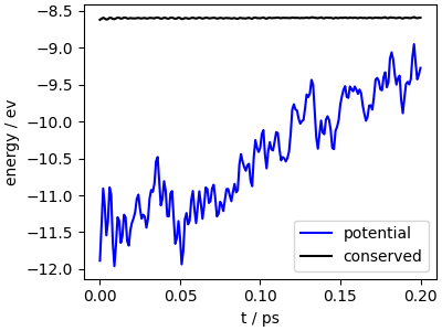
data, info = read_output("qtip4pf-md.out")
trj = read_trajectory("qtip4pf-md.pos_0.xyz")

fig, ax = plt.subplots(1, 1, figsize=(4, 3), constrained_layout=True)

ax.plot(data["time"], data["potential"], "b-", label="potential")
ax.plot(data["time"], data["conserved"] - 4, "k-", label="conserved")
ax.set_xlabel("t / ps")
ax.set_ylabel("energy / ev")
ax.legend()

<matplotlib.legend.Legend object at 0x7f1d75fe8fb0>

chemiscope.show(
    frames=trj,
    properties={
        "time": data["time"][::10],
        "potential": data["potential"][::10],
    },
    mode="default",
    settings=chemiscope.quick_settings(
        map_settings={
            "x": {"property": "time", "scale": "linear"},
            "y": {"property": "potential", "scale": "linear"},
        },
        structure_settings={
            "unitCell": True,
        },
        trajectory=True,
    ),
)

×

Molecular dynamics with LAMMPS

The metatomic model can also be run with LAMMPS and used to perform all kinds of atomistic simulations with it. This only requires defining a pair_metatomic potential, and specifying the mapping between LAMMPS atom types and those used in the model.

Note also that the metatomic interface takes care of converting the model units to those used in the LAMMPS file, so it is possible to use energies in eV even if the model outputs kcal/mol.

with open("data/spcfw.in", "r") as file:
    lines = file.readlines()

for line in lines[:7] + lines[16:]:
    print(line, end="")

units metal  # Angstroms, eV, picoseconds
atom_style atomic
read_data water_32.data

# loads metatomic SPC/Fw model
pair_style metatomic spcfw-mta.pt
pair_coeff * * 1 8

fix 1 all nve
fix 2 all langevin 300 300 1.00 12345

run 200

This specific example runs a short MD trajectory, using a Langevin thermostat. Given that this is a classical MD trajectory, we use the SPC/Fw model that is fitted to reproduce (some) water properties even with a classical description of the nuclei.

We save to geometry to a LAMMPS data file and run the simulation

ase.io.write("water_32.data", atoms, format="lammps-data", masses=True)

subprocess.check_call(["lmp", "-in", "data/spcfw.in"])

0