Hamiltonian Learning for Molecules with Indirect Targets

Authors:

Divya Suman @DivyaSuman14, Hanna Tuerk @HannaTuerk

This tutorial introduces a machine learning (ML) framework that predicts Hamiltonians for molecular systems. Another one of our cookbook examples demonstrates an ML model that predicts real-space Hamiltonians for periodic systems. While we use the same model here to predict a molecular Hamiltonians, we further finetune these models to optimise predictions of different quantum mechanical (QM) properties of interest, thereby treating the Hamiltonian predictions as an intermediate component of the ML framework. More details on this hybrid or indirect learning framework can be found in ACS Cent. Sci. 2024, 10, 637−648. and our preprint arXiv:2504.01187.

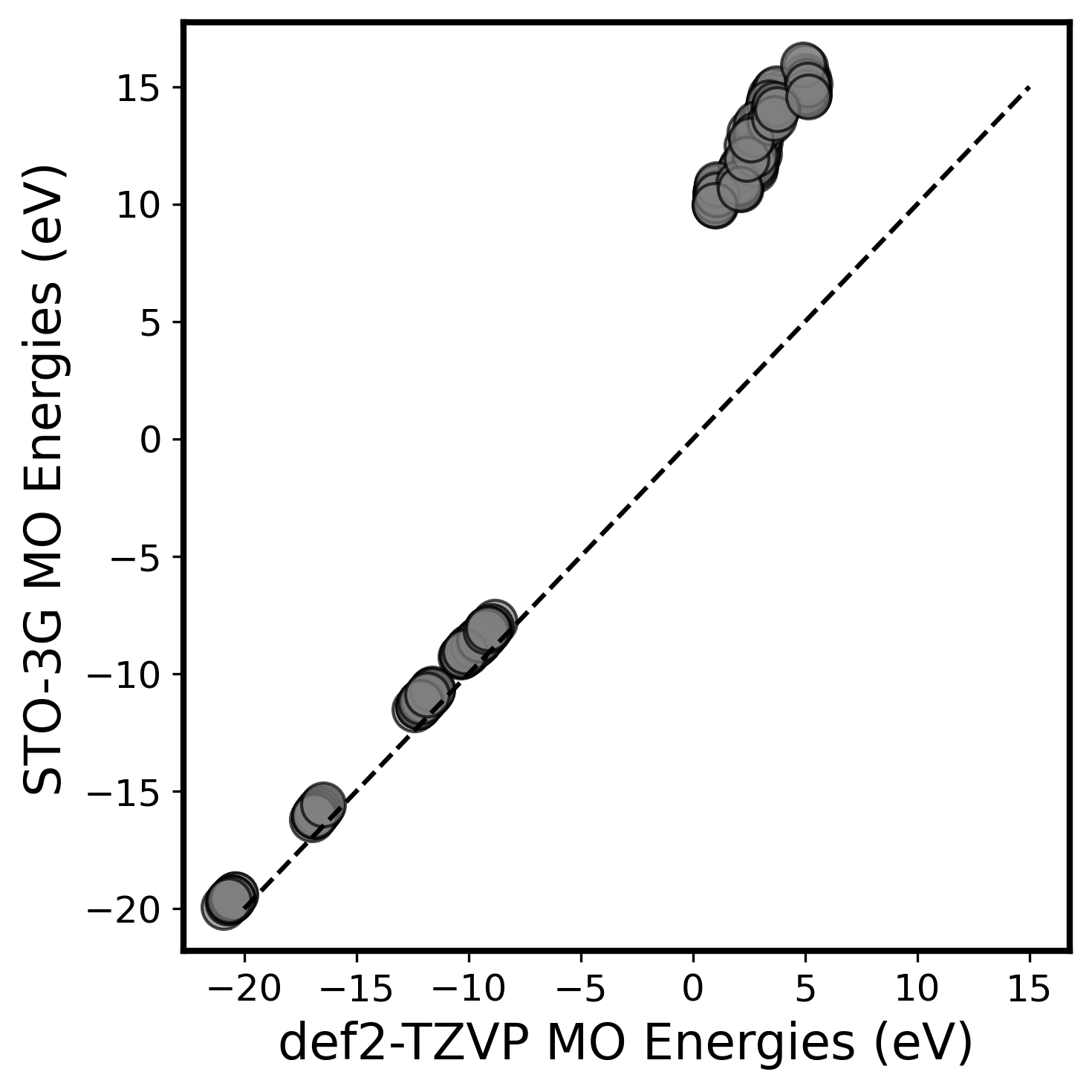
Within a Hamiltonian learning framework, one could chose to learn a target that corresponds to the matrix representation for an existing electronic structure method, but in a finite AO basis, such a representation will lead to a finite basis set error. The parity plot below illustrates this error by showing the discrepancy between molecular orbital (MO) energies of an ethane molecule obtained from a self-consistent calculation on a minimal STO-3G basis and the larger def2-TZVP basis, especially for the high energy, unoccupied MOs.

The choice of basis set plays a crucial role in determining the accuracy of the observables derived from the predicted Hamiltonian. Although the larger basis sets generally provide more reliable results, the computational cost to compute the electronic structure in a larger basis or to train such a model is notably higher compared to a smaller basis. Using the indirect learning framework, one could instead learn a reduced effective Hamiltonian that reproduces calculations from a much larger basis while using a significantly simpler and smaller model consistent with a smaller basis.

We first show an example where we predict the reduced effective Hamiltonians for a homogenous dataset of ethane molecule while targeting the MO energies of the def2-TZVP basis. In a second example we will then target multiple properties for a organic molecule dataset, similar to our results described in our preprint arXiv:2504.01187.

1. Example of Learning MO Energies for Ethane

Python Environment and Used Packages

We start by creating a virtual environment and installing all necessary packages. The required packages are provided in the environment.yml file that can be dowloaded at the end. We can then import the necessary packages.

import os
from zipfile import ZipFile

import matplotlib.pyplot as plt
import numpy as np
import requests
import torch
from ase.units import Hartree
from IPython.utils import io
from mlelec.features.acdc import compute_features_for_target
from mlelec.targets import drop_zero_blocks  # noqa: F401
from mlelec.utils.plot_utils import plot_losses


os.environ["PYSCFAD_BACKEND"] = "torch"
import mlelec.metrics as mlmetrics  # noqa: E402
from mlelec.data.dataset import MLDataset, MoleculeDataset, get_dataloader  # noqa: E402
from mlelec.models.linear import LinearTargetModel  # noqa: E402
from mlelec.train import Trainer  # noqa: E402
from mlelec.utils.property_utils import (  # noqa: E402, F401
    compute_dipole_moment,
    compute_eigvals,
    compute_polarisability,
    instantiate_mf,
)


torch.set_default_dtype(torch.float64)

/home/runner/work/atomistic-cookbook/atomistic-cookbook/.nox/hamiltonian-qm7/lib/python3.11/site-packages/pyscf/dft/libxc.py:772: UserWarning: Since PySCF-2.3, B3LYP (and B3P86) are changed to the VWN-RPA variant, the same to the B3LYP functional in Gaussian and ORCA (issue 1480). To restore the VWN5 definition, you can put the setting "B3LYP_WITH_VWN5 = True" in pyscf_conf.py
  warnings.warn('Since PySCF-2.3, B3LYP (and B3P86) are changed to the VWN-RPA variant, '
Using PyTorch backend.

Set Parameters for Training

Before we begin our training we can decide on a set the parameters, including the dataset set size, splitting fractions, the batch size, learning rate, number of epochs, and the early stop criterion in case of early stopping.

NUM_FRAMES = 100
BATCH_SIZE = 4
NUM_EPOCHS = 100
SHUFFLE_SEED = 42
TRAIN_FRAC = 0.7
TEST_FRAC = 0.1
VALIDATION_FRAC = 0.2
EARLY_STOP_CRITERION = 20
VERBOSE = 10
DUMP_HIST = 50
LR = 1e-1
VAL_INTERVAL = 1
DEVICE = "cpu"

ORTHOGONAL = True  # set to 'FALSE' if working in the non-orthogonal basis
FOLDER_NAME = "output/ethane_eva"
NOISE = False

Create Folders and Save Parameters

We can save the parameters we just defined for our reference later. For this, we create a folder (defined as FOLDER_NAME above) in which all parameters and the generated data for this example are stored.

os.makedirs(FOLDER_NAME, exist_ok=True)
os.makedirs(f"{FOLDER_NAME}/model_output", exist_ok=True)


def save_parameters(file_path, **params):
    with open(file_path, "w") as file:
        for key, value in params.items():
            file.write(f"{key}: {value}\n")


# Call the function with your parameters
save_parameters(
    f"{FOLDER_NAME}/parameters.txt",
    NUM_FRAMES=NUM_FRAMES,
    BATCH_SIZE=BATCH_SIZE,
    NUM_EPOCHS=NUM_EPOCHS,
    SHUFFLE_SEED=SHUFFLE_SEED,
    TRAIN_FRAC=TRAIN_FRAC,
    TEST_FRAC=TEST_FRAC,
    VALIDATION_FRAC=VALIDATION_FRAC,
    LR=LR,
    VAL_INTERVAL=VAL_INTERVAL,
    DEVICE=DEVICE,
    ORTHOGONAL=ORTHOGONAL,
    FOLDER_NAME=FOLDER_NAME,
)

Generate Reference Data

In principle one can generate the training data of reference Hamiltonians from a given set of structures, using any electronic structure code. Here we provide a pre-computed, homogenous dataset that contains 100 different configurations of ethane molecule. For all structures, we performed Kohn-Sham density functional theory (DFT) calculations with PySCF, using the B3LYP functional. For each molecular geometry, we computed the Fock and overlap matrices along with other molecular properties of interest, using both STO-3G and def2-TZVP basis sets.

Download the Dataset from Zenodo

We first download the data for the two examples from Zenodo and unzip the downloaded datafile.

if not os.path.exists("hamiltonian-qm7-data"):
    url = r"https://zenodo.org/records/15524259/files/hamiltonian-qm7-data.zip"
    response = requests.get(url)
    response.raise_for_status()
    with open("hamiltonian-qm7-data.zip", "wb") as f:
        f.write(response.content)

    with ZipFile("hamiltonian-qm7-data.zip", "r") as zObject:
        zObject.extractall(path=".")

Prepare the Dataset for ML Training

In this section, we will prepare the dataset required to train our machine learning model using the MoleculeDataset and MLDataset classes. These classes help format and store the DFT data in a way compatible with our ML package, mlelec. In this section we initialise the MoleculeDataset where we specify the molecule name, file paths and the desired targets and auxillary data to be used for training for the minimal (STO-3G), as well as a larger basis (lb, def2-TZVP). Once the molecular data is prepared, we wrap it into an MLDataset instance. This class structures the dataset into a format that is optimal for ML the Hamiltonians. The Hamiltonian matrix elements depend on specific pairs of orbitals involved in the interaction. When these orbitals are centered on atoms, as is the case for localized AO bases, the Hamiltonian matrix elements can be viewed as objects labeled by pairs of atoms, as well as multiple quantum numbers, namely the radial (n) and the angular (l, m) quantum numbers characterizing each AO. These angular functions are typically chosen to be real spherical harmonics, and determine the equivariant behavior of the matrix elements under rotations and inversions. MLDataset leverages this equivariant structure of the Hamiltonians, which is discussed in further detail in the Periodic Hamiltonian Model Example . Finally, we split the loaded dataset into training, validation and test datasets using _split_indices.

molecule_data = MoleculeDataset(
    mol_name="ethane",
    use_precomputed=False,
    path="hamiltonian-qm7-data/ethane",
    aux_path="hamiltonian-qm7-data/ethane/sto-3g",
    frame_slice=slice(0, NUM_FRAMES),
    device=DEVICE,
    aux=["overlap", "orbitals"],
    lb_aux=["overlap", "orbitals"],
    target=["fock", "eva"],
    lb_target=["fock", "eva"],
)

ml_data = MLDataset(
    molecule_data=molecule_data,
    device=DEVICE,
    model_strategy="coupled",
    shuffle=True,
    shuffle_seed=SHUFFLE_SEED,
    orthogonal=ORTHOGONAL,
)

ml_data._split_indices(
    train_frac=TRAIN_FRAC, val_frac=VALIDATION_FRAC, test_frac=TEST_FRAC
)

Loading structures
hamiltonian-qm7-data/ethane/sto-3g/fock.hickle
hamiltonian-qm7-data/ethane/sto-3g/eva.hickle
hamiltonian-qm7-data/ethane/def2-tzvp/fock.hickle
hamiltonian-qm7-data/ethane/def2-tzvp/eva.hickle
/home/runner/work/atomistic-cookbook/atomistic-cookbook/.nox/hamiltonian-qm7/lib/python3.11/site-packages/mlelec/utils/twocenter_utils.py:78: UserWarning: To copy construct from a tensor, it is recommended to use sourceTensor.detach().clone() or sourceTensor.detach().clone().requires_grad_(True), rather than torch.tensor(sourceTensor).
  return torch.tensor(matrix)[idx][:, idx]

Computing Features that can Learn Hamiltonian Targets

As discussed above, the Hamiltonian matrix elements are dependent on single atom centers and two centers for pairwise interactions. To address this, we extend the equivariant SOAP-based features for the atom-centered desciptors to a descriptor capable of describing multiple atomic centers and their connectivities, giving rise to the equivariant pairwise descriptor which simultaneously characterizes the environments for pairs of atoms in a given system. Our Periodic Hamiltonian Model Example discusses the construction of these descriptors in greater detail. To construct these atom- and pair-centered features we use our in house library featomic for each structure in the our dataset using the hyperparameters defined below. The features are constructed starting from a description of a structure in terms of atom density, for which we define the width of the overlaying Gaussians in the density hyperparameter. The features are discretized on a basis of spherical harmonics, which consist of a radial and an angular part, which can be specified in the basis hyperparameter. The cutoff hyperparameter controls the extent of the atomic environment. For the simple example we demonstrate here, the atom and pairwise features have very similar hyperparameters, except for the cutoff radius, which is larger for pairwise features to include many pairs that describe the individual atom-atom interaction.

hypers = {
    "cutoff": {"radius": 2.5, "smoothing": {"type": "ShiftedCosine", "width": 0.1}},
    "density": {"type": "Gaussian", "width": 0.3},
    "basis": {
        "type": "TensorProduct",
        "max_angular": 4,
        "radial": {"type": "Gto", "max_radial": 5},
    },
}

hypers_pair = {
    "cutoff": {"radius": 3.0, "smoothing": {"type": "ShiftedCosine", "width": 0.1}},
    "density": {"type": "Gaussian", "width": 0.3},
    "basis": {
        "type": "TensorProduct",
        "max_angular": 4,
        "radial": {"type": "Gto", "max_radial": 5},
    },
}

features = compute_features_for_target(
    ml_data, device=DEVICE, hypers=hypers, hypers_pair=hypers_pair
)
ml_data._set_features(features)

Prepare Dataloaders

To efficiently feed data into the model during training, we use data loaders. These handle batching and shuffling to optimize training performance. get_dataloader creates data loaders for training, validation and testing. The model_return="blocks" argument determines that the model targets the different blocks that the Hamiltonian is decomposed into and the batch_size argument defines the number of samples per batch for the batch-wise training.

train_dl, val_dl, test_dl = get_dataloader(
    ml_data, model_return="blocks", batch_size=BATCH_SIZE
)

Prepare Training

Next, we set up our linear model that predicts the Hamiltonian matrices, using LinerTargetModel. To improve the model convergence, we first start with a symmetry-adapted ridge regression targeting the Hamiltonian matrices from the STO-3G basis QM calculation using the fit_ridge_analytical function. This provides us a more reliable set of weights to initialise the fine-tuning rather than starting from any random guess, effectively saving us training time by starting the training process closer to the desired minumum.

model = LinearTargetModel(
    dataset=ml_data, nlayers=1, nhidden=16, bias=False, device=DEVICE
)

pred_ridges, ridges = model.fit_ridge_analytical(
    alpha=np.logspace(-8, 3, 12),
    cv=3,
    set_bias=False,
)

pred_fock = model.forward(
    ml_data.feat_train,
    return_type="tensor",
    batch_indices=ml_data.train_idx,
    ridge_fit=True,
    add_noise=NOISE,
)

with io.capture_output() as captured:
    all_mfs, fockvars = instantiate_mf(
        ml_data,
        fock_predictions=None,
        batch_indices=list(range(len(ml_data.structures))),
    )

Training: Indirect learning of the MO energies

Now rather than explicitly targeting the Hamiltonian matrix, we instead treat it as an intermediate layer in our framework, where the model predicts the Hamiltonian, the model weights, however, are subsequently fine-tuned by backpropagating a loss on a derived molecular property of the Hamiltonian such as the MO energies but from the larger def-TZVP basis instead of the STO-3G basis.

Before fine-tuning the model we preconditioned by a ridge regression fit of our data, we set up the loss function to target the MO energies, as well as the optimizer and the learning rate scheduler for our model. We use a customized mean squared error (MSE) loss function that guides the learning and Adam optimizer that performs a stochastic gradient descent that minimizes the error. The scheduler reduces the learning rate by the given factor if the validation loss plateaus.

loss_fn = mlmetrics.mse_per_atom
optimizer = torch.optim.Adam(model.parameters(), lr=LR)
scheduler = torch.optim.lr_scheduler.ReduceLROnPlateau(
    optimizer,
    factor=0.5,
    patience=3,  # 20,
)

We use a Trainer class to encapsulate all training logic. It manages the training and validation loops.

trainer = Trainer(model, optimizer, scheduler, DEVICE)

Define necessary arguments for the training and validation process.

fit_args = {
    "ml_data": ml_data,
    "all_mfs": all_mfs,
    "loss_fn": loss_fn,
    "weight_eva": 1,
    "weight_dipole": 0,
    "weight_polar": 0,
    "ORTHOGONAL": ORTHOGONAL,
    "upscale": True,
}

With these steps complete, we can now train the model. It begins training and validation using the structured molecular data, features, and defined parameters. The fit function returns the training and validation losses for each epoch, which we can then use to plot the loss versus epoch curve.

history = trainer.fit(
    train_dl,
    val_dl,
    NUM_EPOCHS,
    EARLY_STOP_CRITERION,
    FOLDER_NAME,
    VERBOSE,
    DUMP_HIST,
    **fit_args,
)

np.save(f"{FOLDER_NAME}/model_output/loss_stats.npy", history)

  0%|                                                                                           | 0/100 [00:00<?, ?it/s]
  0%|                                              | 0/100 [00:02<?, ?it/s, train_loss=0.0451, Val_loss=0.00493, lr=0.1]Checkpoint saved to output/ethane_eva/model_output/model_epoch0.pt

  1%|▍                                     | 1/100 [00:03<04:57,  3.00s/it, train_loss=0.0451, Val_loss=0.00493, lr=0.1]
  2%|▊                                     | 2/100 [00:06<04:55,  3.02s/it, train_loss=0.0451, Val_loss=0.00493, lr=0.1]
  3%|█▏                                    | 3/100 [00:09<04:52,  3.02s/it, train_loss=0.0451, Val_loss=0.00493, lr=0.1]
  4%|█▌                                    | 4/100 [00:12<04:50,  3.02s/it, train_loss=0.0451, Val_loss=0.00493, lr=0.1]
  5%|█▉                                    | 5/100 [00:15<04:48,  3.03s/it, train_loss=0.0451, Val_loss=0.00493, lr=0.1]
  6%|██▎                                   | 6/100 [00:18<04:46,  3.05s/it, train_loss=0.0451, Val_loss=0.00493, lr=0.1]
  7%|██▋                                   | 7/100 [00:21<04:42,  3.04s/it, train_loss=0.0451, Val_loss=0.00493, lr=0.1]
  8%|███                                   | 8/100 [00:24<04:39,  3.04s/it, train_loss=0.0451, Val_loss=0.00493, lr=0.1]
  9%|███▍                                  | 9/100 [00:27<04:37,  3.05s/it, train_loss=0.0451, Val_loss=0.00493, lr=0.1]
 10%|███▋                                 | 10/100 [00:30<04:35,  3.06s/it, train_loss=0.0451, Val_loss=0.00493, lr=0.1]
 10%|███▌                                | 10/100 [00:33<04:35,  3.06s/it, train_loss=6.43e-6, Val_loss=7.19e-6, lr=0.1]
 11%|███▉                                | 11/100 [00:33<04:29,  3.03s/it, train_loss=6.43e-6, Val_loss=7.19e-6, lr=0.1]
 12%|████▎                               | 12/100 [00:36<04:25,  3.02s/it, train_loss=6.43e-6, Val_loss=7.19e-6, lr=0.1]
 13%|████▋                               | 13/100 [00:39<04:21,  3.01s/it, train_loss=6.43e-6, Val_loss=7.19e-6, lr=0.1]
 14%|█████                               | 14/100 [00:42<04:18,  3.00s/it, train_loss=6.43e-6, Val_loss=7.19e-6, lr=0.1]
 15%|█████▍                              | 15/100 [00:45<04:15,  3.01s/it, train_loss=6.43e-6, Val_loss=7.19e-6, lr=0.1]
 16%|█████▊                              | 16/100 [00:48<04:13,  3.02s/it, train_loss=6.43e-6, Val_loss=7.19e-6, lr=0.1]
 17%|██████                              | 17/100 [00:51<04:12,  3.04s/it, train_loss=6.43e-6, Val_loss=7.19e-6, lr=0.1]
 18%|██████▍                             | 18/100 [00:54<04:09,  3.04s/it, train_loss=6.43e-6, Val_loss=7.19e-6, lr=0.1]
 19%|██████▊                             | 19/100 [00:57<04:07,  3.05s/it, train_loss=6.43e-6, Val_loss=7.19e-6, lr=0.1]
 20%|███████▏                            | 20/100 [01:00<04:04,  3.05s/it, train_loss=6.43e-6, Val_loss=7.19e-6, lr=0.1]
 20%|███████▏                            | 20/100 [01:03<04:04,  3.05s/it, train_loss=4.34e-6, Val_loss=4.5e-6, lr=0.05]
 21%|███████▌                            | 21/100 [01:03<04:00,  3.04s/it, train_loss=4.34e-6, Val_loss=4.5e-6, lr=0.05]
 22%|███████▉                            | 22/100 [01:06<03:57,  3.04s/it, train_loss=4.34e-6, Val_loss=4.5e-6, lr=0.05]
 23%|████████▎                           | 23/100 [01:09<03:54,  3.04s/it, train_loss=4.34e-6, Val_loss=4.5e-6, lr=0.05]
 24%|████████▋                           | 24/100 [01:12<03:50,  3.03s/it, train_loss=4.34e-6, Val_loss=4.5e-6, lr=0.05]
 25%|█████████                           | 25/100 [01:15<03:42,  2.97s/it, train_loss=4.34e-6, Val_loss=4.5e-6, lr=0.05]
 26%|█████████▎                          | 26/100 [01:18<03:40,  2.98s/it, train_loss=4.34e-6, Val_loss=4.5e-6, lr=0.05]
 27%|█████████▋                          | 27/100 [01:21<03:37,  2.99s/it, train_loss=4.34e-6, Val_loss=4.5e-6, lr=0.05]
 28%|██████████                          | 28/100 [01:24<03:36,  3.00s/it, train_loss=4.34e-6, Val_loss=4.5e-6, lr=0.05]
 29%|██████████▍                         | 29/100 [01:27<03:33,  3.01s/it, train_loss=4.34e-6, Val_loss=4.5e-6, lr=0.05]
 30%|██████████▊                         | 30/100 [01:30<03:31,  3.03s/it, train_loss=4.34e-6, Val_loss=4.5e-6, lr=0.05]
 30%|██████████▏                       | 30/100 [01:33<03:31,  3.03s/it, train_loss=2.98e-6, Val_loss=3.12e-6, lr=0.025]
 31%|██████████▌                       | 31/100 [01:33<03:28,  3.02s/it, train_loss=2.98e-6, Val_loss=3.12e-6, lr=0.025]
 32%|██████████▉                       | 32/100 [01:36<03:24,  3.01s/it, train_loss=2.98e-6, Val_loss=3.12e-6, lr=0.025]
 33%|███████████▏                      | 33/100 [01:39<03:20,  2.99s/it, train_loss=2.98e-6, Val_loss=3.12e-6, lr=0.025]
 34%|███████████▌                      | 34/100 [01:42<03:17,  2.99s/it, train_loss=2.98e-6, Val_loss=3.12e-6, lr=0.025]
 35%|███████████▉                      | 35/100 [01:45<03:14,  2.99s/it, train_loss=2.98e-6, Val_loss=3.12e-6, lr=0.025]
 36%|████████████▏                     | 36/100 [01:48<03:11,  2.99s/it, train_loss=2.98e-6, Val_loss=3.12e-6, lr=0.025]
 37%|████████████▌                     | 37/100 [01:51<03:10,  3.02s/it, train_loss=2.98e-6, Val_loss=3.12e-6, lr=0.025]
 38%|████████████▉                     | 38/100 [01:54<03:07,  3.02s/it, train_loss=2.98e-6, Val_loss=3.12e-6, lr=0.025]
 39%|█████████████▎                    | 39/100 [01:57<03:04,  3.02s/it, train_loss=2.98e-6, Val_loss=3.12e-6, lr=0.025]
 40%|█████████████▌                    | 40/100 [02:00<03:01,  3.02s/it, train_loss=2.98e-6, Val_loss=3.12e-6, lr=0.025]
 40%|██████████████                     | 40/100 [02:03<03:01,  3.02s/it, train_loss=3.5e-6, Val_loss=4.43e-6, lr=0.025]
 41%|██████████████▎                    | 41/100 [02:03<02:58,  3.02s/it, train_loss=3.5e-6, Val_loss=4.43e-6, lr=0.025]
 42%|██████████████▋                    | 42/100 [02:06<02:54,  3.01s/it, train_loss=3.5e-6, Val_loss=4.43e-6, lr=0.025]
 43%|███████████████                    | 43/100 [02:09<02:51,  3.01s/it, train_loss=3.5e-6, Val_loss=4.43e-6, lr=0.025]
 44%|███████████████▍                   | 44/100 [02:12<02:48,  3.01s/it, train_loss=3.5e-6, Val_loss=4.43e-6, lr=0.025]
 45%|███████████████▊                   | 45/100 [02:15<02:45,  3.01s/it, train_loss=3.5e-6, Val_loss=4.43e-6, lr=0.025]
 46%|████████████████                   | 46/100 [02:18<02:42,  3.01s/it, train_loss=3.5e-6, Val_loss=4.43e-6, lr=0.025]
 47%|████████████████▍                  | 47/100 [02:21<02:39,  3.01s/it, train_loss=3.5e-6, Val_loss=4.43e-6, lr=0.025]
 48%|████████████████▊                  | 48/100 [02:24<02:36,  3.02s/it, train_loss=3.5e-6, Val_loss=4.43e-6, lr=0.025]
 49%|█████████████████▏                 | 49/100 [02:27<02:33,  3.01s/it, train_loss=3.5e-6, Val_loss=4.43e-6, lr=0.025]
 50%|█████████████████▌                 | 50/100 [02:30<02:30,  3.01s/it, train_loss=3.5e-6, Val_loss=4.43e-6, lr=0.025]
 50%|████████████████▌                | 50/100 [02:33<02:30,  3.01s/it, train_loss=2.52e-6, Val_loss=2.82e-6, lr=0.0125]Checkpoint saved to output/ethane_eva/model_output/model_epoch50.pt

 51%|████████████████▊                | 51/100 [02:33<02:27,  3.02s/it, train_loss=2.52e-6, Val_loss=2.82e-6, lr=0.0125]
 52%|█████████████████▏               | 52/100 [02:36<02:24,  3.00s/it, train_loss=2.52e-6, Val_loss=2.82e-6, lr=0.0125]
 53%|█████████████████▍               | 53/100 [02:39<02:21,  3.01s/it, train_loss=2.52e-6, Val_loss=2.82e-6, lr=0.0125]
 54%|█████████████████▊               | 54/100 [02:42<02:15,  2.95s/it, train_loss=2.52e-6, Val_loss=2.82e-6, lr=0.0125]
 55%|██████████████████▏              | 55/100 [02:45<02:13,  2.96s/it, train_loss=2.52e-6, Val_loss=2.82e-6, lr=0.0125]
 56%|██████████████████▍              | 56/100 [02:48<02:10,  2.98s/it, train_loss=2.52e-6, Val_loss=2.82e-6, lr=0.0125]
 57%|██████████████████▊              | 57/100 [02:51<02:08,  2.99s/it, train_loss=2.52e-6, Val_loss=2.82e-6, lr=0.0125]
 58%|███████████████████▏             | 58/100 [02:54<02:05,  2.99s/it, train_loss=2.52e-6, Val_loss=2.82e-6, lr=0.0125]
 59%|███████████████████▍             | 59/100 [02:57<02:02,  3.00s/it, train_loss=2.52e-6, Val_loss=2.82e-6, lr=0.0125]
 60%|███████████████████▊             | 60/100 [03:00<02:00,  3.00s/it, train_loss=2.52e-6, Val_loss=2.82e-6, lr=0.0125]
 60%|███████████████████▏            | 60/100 [03:03<02:00,  3.00s/it, train_loss=2.34e-6, Val_loss=2.25e-6, lr=0.00625]
 61%|███████████████████▌            | 61/100 [03:03<01:56,  3.00s/it, train_loss=2.34e-6, Val_loss=2.25e-6, lr=0.00625]
 62%|███████████████████▊            | 62/100 [03:06<01:53,  3.00s/it, train_loss=2.34e-6, Val_loss=2.25e-6, lr=0.00625]
 63%|████████████████████▏           | 63/100 [03:09<01:51,  3.01s/it, train_loss=2.34e-6, Val_loss=2.25e-6, lr=0.00625]
 64%|████████████████████▍           | 64/100 [03:12<01:48,  3.00s/it, train_loss=2.34e-6, Val_loss=2.25e-6, lr=0.00625]
 65%|████████████████████▊           | 65/100 [03:15<01:44,  3.00s/it, train_loss=2.34e-6, Val_loss=2.25e-6, lr=0.00625]
 66%|█████████████████████           | 66/100 [03:18<01:41,  3.00s/it, train_loss=2.34e-6, Val_loss=2.25e-6, lr=0.00625]
 67%|█████████████████████▍          | 67/100 [03:21<01:38,  2.99s/it, train_loss=2.34e-6, Val_loss=2.25e-6, lr=0.00625]
 68%|█████████████████████▊          | 68/100 [03:24<01:35,  2.98s/it, train_loss=2.34e-6, Val_loss=2.25e-6, lr=0.00625]
 69%|██████████████████████          | 69/100 [03:27<01:32,  2.99s/it, train_loss=2.34e-6, Val_loss=2.25e-6, lr=0.00625]
 70%|██████████████████████▍         | 70/100 [03:30<01:29,  2.99s/it, train_loss=2.34e-6, Val_loss=2.25e-6, lr=0.00625]
 70%|███████████████████████          | 70/100 [03:33<01:29,  2.99s/it, train_loss=2.07e-6, Val_loss=2.1e-6, lr=0.00313]
 71%|███████████████████████▍         | 71/100 [03:33<01:26,  2.97s/it, train_loss=2.07e-6, Val_loss=2.1e-6, lr=0.00313]
 72%|███████████████████████▊         | 72/100 [03:36<01:23,  2.97s/it, train_loss=2.07e-6, Val_loss=2.1e-6, lr=0.00313]
 73%|████████████████████████         | 73/100 [03:39<01:20,  2.97s/it, train_loss=2.07e-6, Val_loss=2.1e-6, lr=0.00313]
 74%|████████████████████████▍        | 74/100 [03:42<01:17,  2.98s/it, train_loss=2.07e-6, Val_loss=2.1e-6, lr=0.00313]
 75%|████████████████████████▊        | 75/100 [03:45<01:14,  2.98s/it, train_loss=2.07e-6, Val_loss=2.1e-6, lr=0.00313]
 76%|█████████████████████████        | 76/100 [03:48<01:11,  2.98s/it, train_loss=2.07e-6, Val_loss=2.1e-6, lr=0.00313]
 77%|█████████████████████████▍       | 77/100 [03:51<01:08,  2.97s/it, train_loss=2.07e-6, Val_loss=2.1e-6, lr=0.00313]
 78%|█████████████████████████▋       | 78/100 [03:54<01:05,  2.96s/it, train_loss=2.07e-6, Val_loss=2.1e-6, lr=0.00313]
 79%|██████████████████████████       | 79/100 [03:57<01:00,  2.90s/it, train_loss=2.07e-6, Val_loss=2.1e-6, lr=0.00313]
 80%|██████████████████████████▍      | 80/100 [04:00<00:58,  2.92s/it, train_loss=2.07e-6, Val_loss=2.1e-6, lr=0.00313]
 80%|██████████████████████████▍      | 80/100 [04:03<00:58,  2.92s/it, train_loss=2.06e-6, Val_loss=2.2e-6, lr=0.00313]
 81%|██████████████████████████▋      | 81/100 [04:03<00:55,  2.92s/it, train_loss=2.06e-6, Val_loss=2.2e-6, lr=0.00313]
 82%|███████████████████████████      | 82/100 [04:06<00:52,  2.94s/it, train_loss=2.06e-6, Val_loss=2.2e-6, lr=0.00313]
 83%|███████████████████████████▍     | 83/100 [04:09<00:50,  2.96s/it, train_loss=2.06e-6, Val_loss=2.2e-6, lr=0.00313]
 84%|███████████████████████████▋     | 84/100 [04:11<00:47,  2.95s/it, train_loss=2.06e-6, Val_loss=2.2e-6, lr=0.00313]
 85%|████████████████████████████     | 85/100 [04:14<00:44,  2.95s/it, train_loss=2.06e-6, Val_loss=2.2e-6, lr=0.00313]
 86%|████████████████████████████▍    | 86/100 [04:17<00:41,  2.95s/it, train_loss=2.06e-6, Val_loss=2.2e-6, lr=0.00313]
 87%|████████████████████████████▋    | 87/100 [04:20<00:38,  2.94s/it, train_loss=2.06e-6, Val_loss=2.2e-6, lr=0.00313]
 88%|█████████████████████████████    | 88/100 [04:23<00:35,  2.92s/it, train_loss=2.06e-6, Val_loss=2.2e-6, lr=0.00313]
 89%|█████████████████████████████▎   | 89/100 [04:26<00:32,  2.92s/it, train_loss=2.06e-6, Val_loss=2.2e-6, lr=0.00313]
 90%|█████████████████████████████▋   | 90/100 [04:29<00:29,  2.92s/it, train_loss=2.06e-6, Val_loss=2.2e-6, lr=0.00313]
 90%|████████████████████████████▊   | 90/100 [04:32<00:29,  2.92s/it, train_loss=1.86e-6, Val_loss=1.96e-6, lr=0.00313]
 91%|█████████████████████████████   | 91/100 [04:32<00:26,  2.92s/it, train_loss=1.86e-6, Val_loss=1.96e-6, lr=0.00313]
 92%|█████████████████████████████▍  | 92/100 [04:35<00:23,  2.93s/it, train_loss=1.86e-6, Val_loss=1.96e-6, lr=0.00313]
 93%|█████████████████████████████▊  | 93/100 [04:38<00:20,  2.93s/it, train_loss=1.86e-6, Val_loss=1.96e-6, lr=0.00313]
 94%|██████████████████████████████  | 94/100 [04:41<00:17,  2.93s/it, train_loss=1.86e-6, Val_loss=1.96e-6, lr=0.00313]
 95%|██████████████████████████████▍ | 95/100 [04:44<00:14,  2.93s/it, train_loss=1.86e-6, Val_loss=1.96e-6, lr=0.00313]
 96%|██████████████████████████████▋ | 96/100 [04:47<00:11,  2.93s/it, train_loss=1.86e-6, Val_loss=1.96e-6, lr=0.00313]
 97%|███████████████████████████████ | 97/100 [04:50<00:08,  2.94s/it, train_loss=1.86e-6, Val_loss=1.96e-6, lr=0.00313]
 98%|███████████████████████████████▎| 98/100 [04:52<00:05,  2.93s/it, train_loss=1.86e-6, Val_loss=1.96e-6, lr=0.00313]
 99%|███████████████████████████████▋| 99/100 [04:55<00:02,  2.93s/it, train_loss=1.86e-6, Val_loss=1.96e-6, lr=0.00313]
100%|███████████████████████████████| 100/100 [04:58<00:00,  2.93s/it, train_loss=1.86e-6, Val_loss=1.96e-6, lr=0.00313]
100%|███████████████████████████████| 100/100 [04:58<00:00,  2.99s/it, train_loss=1.86e-6, Val_loss=1.96e-6, lr=0.00313]

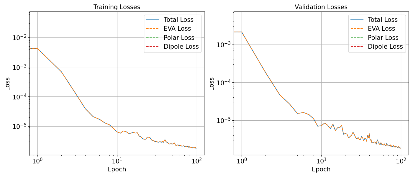
Plot Loss

With the help of plot_losses function we can conveniently plot the training and validation losses.

plot_losses(history, save=True, savename=f"{FOLDER_NAME}/loss_vs_epoch.pdf")

Parity Plot

We then evaluate the prediction of the fine-tuned model on the MO energies by comparing it the with the MO energies from the reference def2-TZVP calculation.

f_pred = model.forward(
    ml_data.feat_test,
    return_type="tensor",
    batch_indices=ml_data.test_idx,
)

test_eva_pred = compute_eigvals(
    ml_data, f_pred, range(len(ml_data.test_idx)), orthogonal=ORTHOGONAL
)

# The parity plot
# below shows the performance of our model on the test
# dataset. ML predictions are shown with blue points and
# the corresponding MO energies from the STO-3G basis are
# are shown in grey.


def plot_parity_properties(
    molecule_data,
    ml_data,
    Hartree,
    properties="eva",  # can be single string or list of strings
    predictions_dict=None,  # dictionary with keys: "eva", "dip", "pol"
):
    # Labels, units, and axis ranges
    prop_info_map = {
        "eva": {"label": "MO Energies", "unit": "eV", "range": [-35, 30]},
        "dip": {"label": "dipoles", "unit": "a.u.", "range": [-2.5, 3]},
        "pol": {"label": "polarisability", "unit": "a.u.", "range": [-25, 150]},
    }

    if type(properties) is list:
        n = len(properties)
    elif type(properties) is str:
        properties = [properties]
        n = 1
    else:
        print("Properties input should be string or list")

    fig, axes = plt.subplots(1, n, figsize=(6 * n, 6))
    if type(axes) is not list:
        axes = [axes]  # Make iterable

    for i, propert in enumerate(properties):
        ax = axes[i]
        label = prop_info_map[propert]["label"]
        unit = prop_info_map[propert]["unit"]
        min_val, max_val = prop_info_map[propert]["range"]

        ax.set_axisbelow(True)
        ax.grid(True, which="both", linestyle="-", linewidth=1, alpha=0.7)
        ax.plot(
            [min_val, max_val],
            [min_val, max_val],
            linestyle="--",
            color="black",
            linewidth=1.5,
        )

        # Reference vs low-basis
        target_vals = []
        lb_vals = []

        for idx in ml_data.test_idx:
            target = molecule_data.target[propert][idx]
            lb = molecule_data.lb_target[propert][idx]
            if propert == "eva":
                lb = lb[: target.shape[0]]
            target_vals.append(target)
            lb_vals.append(lb)

        target_tensor = torch.cat(target_vals)
        lb_tensor = torch.cat(lb_vals)
        x_vals = lb_tensor.detach().numpy().flatten()
        y_vals = target_tensor.detach().numpy().flatten()

        if propert == "eva":
            x_vals *= Hartree
            y_vals *= Hartree

        ax.scatter(
            x_vals,
            y_vals,
            color="gray",
            alpha=0.7,
            s=200,
            marker="o",
            edgecolor="black",
            label="STO-3G",
        )

        # Use saved predictions
        pred_array = predictions_dict[propert]
        if propert == "eva":
            pred_array = np.concatenate(
                [p[: t.shape[0]] for p, t in zip(pred_array, target_vals)]
            )
            y_model = pred_array * Hartree
            x_model = x_vals
        elif propert == "dip":
            y_model = pred_array
            x_model = x_vals
        elif propert == "pol":
            y_model = pred_array
            x_model = x_vals
        else:
            print(f"Unknown property: {propert}")
            continue

        ax.scatter(
            x_model,
            y_model,
            color="royalblue",
            alpha=0.7,
            s=200,
            marker="o",
            edgecolor="black",
            label=r"indirect $\mathbf{H}$ model",
        )

        ax.set_xlabel(f"Target {label} ({unit})", fontsize=16, fontweight="bold")
        ax.set_ylabel(f"Predicted {label} ({unit})", fontsize=16, fontweight="bold")
        ax.set_xlim(min_val, max_val)
        ax.set_ylim(min_val, max_val)
        ax.legend(fontsize=14)

    plt.tight_layout()
    # plt.savefig(f"{FOLDER_NAME}/parity_combined.png", bbox_inches="tight", dpi=300)
    plt.show()


predictions_dict = {
    "eva": [p.detach().numpy() for p in test_eva_pred],
}
plot_parity_properties(
    molecule_data,
    ml_data,
    Hartree,
    properties=["eva"],
    predictions_dict=predictions_dict,
)

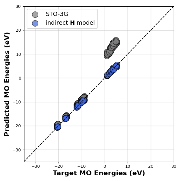
We can observe from the parity plot that even with a minimal basis parametrisation, the model is able to reproduce the large basis MO energies with good accuracy. Thus, using an indirect model, makes it possible to promote the model accuracy to a higher level of theory, at no additional cost.

2. Example of Targeting Multiple Properties

In principle we can also target multiple properties for the indirect training. While MO energies can be computed by simply diagonalizing the Hamiltonian matrix, some properties like the dipole moment require the position operator integral and its derivative if we want to backpropagate the loss. We therefore interface our ML model with an electronic structure code that supports automatic differentiation, PySCFAD, an end-to-end auto-differentiable version of PySCF. By doing so we delegate the computation of properties to PySCFAD, which provides automatic differentiation of observables with respect to the intermediate Hamiltonian. In particular, we will now indirectly target the dipole moment and polarisability along with the MO energies from a large basis reference calculation

Get Data and Prepare Data Set

In our last example even though we show an indirect ML model that was trained on a homogenous dataset of different configurations of ethane, we can also easily extend the framework to use a much diverse dataset such as the QM7 dataset. For our next example we select a subset of 150 structures from this dataset that consists of only C, H, N and O atoms.

Set parameters for training

Set the parameters for the training, including the dataset set size and split, the batch size, learning rate and weights for the individual components of eigenvalues, dipole and polarisability. We additionally define a folder name, in which the results are saved. Optionally, noise can be added to the ridge regression fit.

Here, we now need to provide different weights for the different targets (eigenvalues \(\epsilon\), the dipole moment \(\mu\), and polarisability \(\alpha\)), which we will use when computing the loss \(\mathcal{L}\).

\[\begin{split}\mathcal{L}_{\epsilon,\mu,\alpha} = & \; \frac{\omega_{\epsilon}}{N} \sum_{n=1}^{N} \frac{1}{O_n} \ \sum_{o=1}^{O_n} \left( \epsilon_{no} - \tilde{\epsilon}_{no} \right)^2 \ + \frac{\omega_{\mu}}{N} \sum_{n=1}^{N} \frac{1}{N_A^2} \ \sum_{m=1}^{N_A} \left( \mu_{nm} - \tilde{\mu}_{nm} \right)^2 \\ & + \frac{\omega_{\alpha}}{N} \sum_{n=1}^{N} \frac{1}{N_A^2} \ \sum_{m=1}^{N_A} \left( \alpha_{nm} - \tilde{\alpha}_{nm} \right)^2\end{split}\]

where \(N\) is the number of training points, \(O_n\) is the number of MO orbitals in the nth molecule, \(N_A\) is the number of atoms \(i\).

The weights \(\omega\) in the loss are based on the magnitude of errors for different properties, where at the end we want each of them to contribute equally to the loss. The following values worked well for the QM7 example, but of course depending on the system that one investigates another set of weights might work better.

NUM_FRAMES = 150
LR = 1e-3
W_EVA = 1e4
W_DIP = 1e3
W_POL = 1e2

FOLDER_NAME = "output/qm7"

Create Datasets

We use the dataloader of the mlelec package (qm7 branch), and load the QM7 dataset we downloaded above from zenodo for the defined number of frames. First, we load all relavant data (geometric structures, auxiliary matrices -overlap and orbitals-, and targets -fock, dipole moment, and polarisablity-) into a molecule dataset. We do this for the minimal (STO-3G), as well as a larger basis (lb, def2-TZVP). The larger basis has additional basis functions on the valence electrons. The dataset, we can then load into our dataloader `ml_data`, together with some settings on how we want to sample data from the dataloader. Finally, we define the desired dataset split for training, validation, and testing from the parameters defined in example 1.

molecule_data = MoleculeDataset(
    mol_name="qm7",
    use_precomputed=False,
    path="hamiltonian-qm7-data/qm7",
    aux_path="hamiltonian-qm7-data/qm7/sto-3g",
    frame_slice=slice(0, NUM_FRAMES),
    device=DEVICE,
    aux=["overlap", "orbitals"],
    lb_aux=["overlap", "orbitals"],
    target=["fock", "eva", "dip", "pol"],
    lb_target=["fock", "eva", "dip", "pol"],
)

ml_data = MLDataset(
    molecule_data=molecule_data,
    device=DEVICE,
    model_strategy="coupled",
    shuffle=True,
    shuffle_seed=SHUFFLE_SEED,
    orthogonal=ORTHOGONAL,
)

ml_data._split_indices(
    train_frac=TRAIN_FRAC, val_frac=VALIDATION_FRAC, test_frac=TEST_FRAC
)

Loading structures
hamiltonian-qm7-data/qm7/sto-3g/fock.hickle
hamiltonian-qm7-data/qm7/sto-3g/eva.hickle
hamiltonian-qm7-data/qm7/sto-3g/dip.hickle
hamiltonian-qm7-data/qm7/sto-3g/pol.hickle
hamiltonian-qm7-data/qm7/def2-tzvp/fock.hickle
hamiltonian-qm7-data/qm7/def2-tzvp/eva.hickle
hamiltonian-qm7-data/qm7/def2-tzvp/dip.hickle
hamiltonian-qm7-data/qm7/def2-tzvp/pol.hickle
/home/runner/work/atomistic-cookbook/atomistic-cookbook/.nox/hamiltonian-qm7/lib/python3.11/site-packages/mlelec/utils/twocenter_utils.py:78: UserWarning: To copy construct from a tensor, it is recommended to use sourceTensor.detach().clone() or sourceTensor.detach().clone().requires_grad_(True), rather than torch.tensor(sourceTensor).
  return torch.tensor(matrix)[idx][:, idx]

Compute Features

The feature hyperparameters here are similar to the ones we used for our previous training, except the cutoff. For a dataset like QM7 which contains molecules with over 15 atoms, we need a slightly larger cutoff than the ones we used in case of ethane. We choose a cutoff of 3 and 5 for the atom-centred and pair-centred features, respectively. Note that the computation of the features takes some time and requires a large amount of memory.

This is why in the following of this example, we are not executing the commands related to the features (that is feature computation, training, and evaluation), but provide all python commands necessary if one would want to do this.

hypers = {
    "cutoff": {"radius": 3, "smoothing": {"type": "ShiftedCosine", "width": 0.1}},
    "density": {"type": "Gaussian", "width": 0.3},
    "basis": {
        "type": "TensorProduct",
        "max_angular": 4,
        "radial": {"type": "Gto", "max_radial": 5},
    },
}

hypers_pair = {
    "cutoff": {"radius": 5, "smoothing": {"type": "ShiftedCosine", "width": 0.1}},
    "density": {"type": "Gaussian", "width": 0.3},
    "basis": {
        "type": "TensorProduct",
        "max_angular": 4,
        "radial": {"type": "Gto", "max_radial": 5},
    },
}

features = compute_features_for_target(
    ml_data, device=DEVICE, hypers=hypers, hypers_pair=hypers_pair
)
ml_data._set_features(features)

train_dl, val_dl, test_dl = get_dataloader(
    ml_data, model_return="blocks", batch_size=BATCH_SIZE
)

Depending on the diversity of the structures in the datasets, it may happen that some blocks are empty, because certain structural features are only present in certain structures (e.g. if we would have some organic molecules with oxygen and some without). As this is the case for the QM7 example, we drop these blocks, so that the dataloader does not try to load them during training.

ml_data.target_train, ml_data.target_val, ml_data.target_test = drop_zero_blocks(
ml_data.target_train, ml_data.target_val, ml_data.target_test)

ml_data.feat_train, ml_data.feat_val, ml_data.feat_test = drop_zero_blocks(
ml_data.feat_train, ml_data.feat_val, ml_data.feat_test)

Prepare training

Here again we first fit a ridge regression model to the data.

model = LinearTargetModel(
    dataset=ml_data, nlayers=1, nhidden=16, bias=False, device=DEVICE
)

pred_ridges, ridges = model.fit_ridge_analytical(
    alpha=np.logspace(-8, 3, 12),
    cv=3,
    set_bias=False,
)

pred_fock = model.forward(
    ml_data.feat_train,
    return_type="tensor",
    batch_indices=ml_data.train_idx,
    ridge_fit=True,
    add_noise=NOISE,
)

with io.capture_output() as captured:
    all_mfs, fockvars = instantiate_mf(
        ml_data,
        fock_predictions=None,
        batch_indices=list(range(len(ml_data.structures))),
    )

Training parameters and training

For finetuning on multiple targets we again define a loss function, optimizer and scheduler. We also define the necessary arguments for training and validation.

loss_fn = mlmetrics.mse_per_atom
optimizer = torch.optim.Adam(model.parameters(), lr=LR)
scheduler = torch.optim.lr_scheduler.ReduceLROnPlateau(
    optimizer,
    factor=0.5,
    patience=10,
    )

# Initialize trainer
trainer = Trainer(model, optimizer, scheduler, DEVICE)

# Define necessary arguments for the training and validation process
fit_args = {
    "ml_data": ml_data,
    "all_mfs": all_mfs,
    "loss_fn": loss_fn,
    "weight_eva": W_EVA,
    "weight_dipole": W_DIP,
    "weight_polar": W_POL,
    "ORTHOGONAL": ORTHOGONAL,
    "upscale": True,
}


# Train and validate
history = trainer.fit(
    train_dl,
    val_dl,
    200,
    EARLY_STOP_CRITERION,
    FOLDER_NAME,
    VERBOSE,
    DUMP_HIST,
    **fit_args,
)

# Save the loss history
np.save(f"{FOLDER_NAME}/model_output/loss_stats.npy", history)

This training can take some time to converge fully. Thus, for this example, we load a previously trained model to continue.

Evaluating the trained model

A previously trained model for the QM7 dataset we are using here is also part of the data downloaded from Zenodo.

model.load_state_dict(torch.load("hamiltonian-qm7-data/qm7/output/qm7_eva_dip_pol/best_model.pt"))

We can then compute different properties from the trained model.

batch_indices = ml_data.test_idx
test_fock_predictions = model.forward(
    ml_data.feat_test,
    return_type="tensor",
    batch_indices=ml_data.test_idx,
)
test_dip_pred, test_polar_pred, test_eva_pred = (
    compute_batch_polarisability(
         ml_data,
        test_fock_predictions,
        batch_indices=batch_indices,
        mfs=all_mfs,
        orthogonal=ORTHOGONAL,
    )
)

Plot loss

As we have not performed training, we cannot plot the training and validation losses from the history, as we did for example 1. In principle, if training would have been performed, the python command would be the same:

plot_losses(history, save=True, savename=f"{FOLDER_NAME}/loss_vs_epoch.pdf")

For reference, we provide the loss plot we obtained during training of the saved model that we load above.

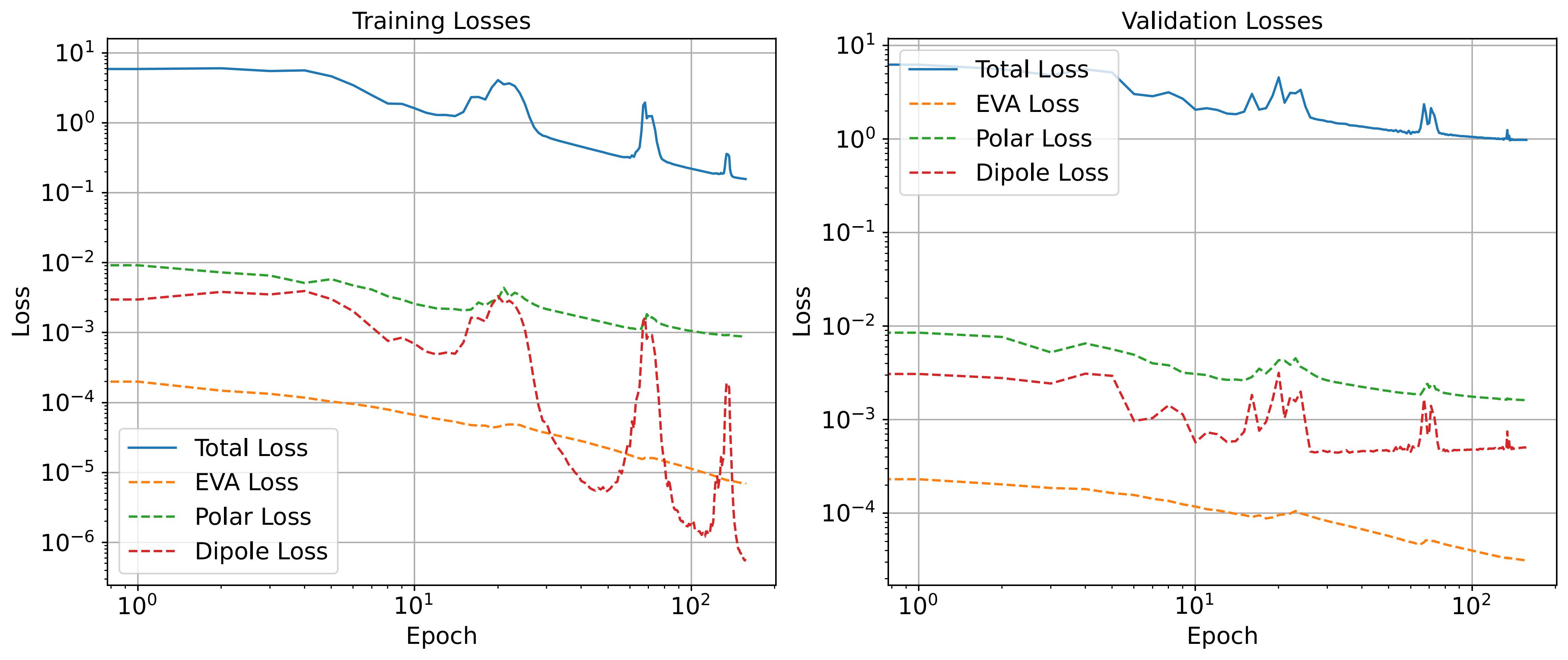
The plot shows the Loss versus Epoch curves for training and validation losses. The MSE on MO energies, dipole moments and polarisability are shown separately.

Parity plot

We finally want to investigate the performance of the finetuned model that target the MO energies, dipole moments and polarisibaility of from a def2-TZVP calculation on the QM7 test dataset. This can be done with the following python command:

predictions_dict = {
    "eva": [p.detach().numpy() for p in test_eva_pred],
    "dip": test_dip_pred.detach().numpy(),
    "pol": test_polar_pred.detach().numpy(),
}

plot_parity_properties(
    molecule_data,
    ml_data,
    Hartree,
    properties=["eva", "dip", "pol"],
    predictions_dict=predictions_dict
)

This command generates a parity plot for the desired properties. As we did not compute the features of the QM7 dataset for time and memory reasons, we do here not execute the python command above but provide directly the parity plot as Figure.

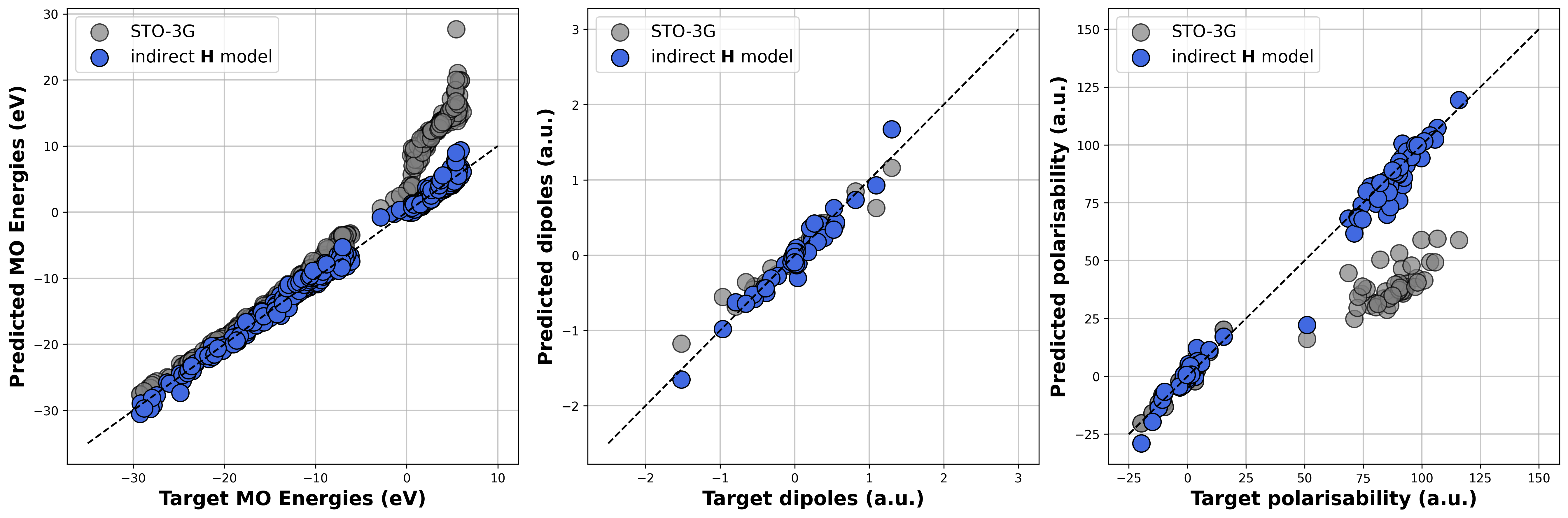
Gray circles correspond to the values obtained from STO-3G calculations, while the blue ones correspond to values computed from the reduced-basis Hamiltonians predicted by the ML model.