Equivariant model for tensorial properties based on scalar features

Authors:

Paolo Pegolo @ppegolo

In this example, we demonstrate how to train a metatensor atomistic model on dipole moments and polarizabilities of small molecular systems, using a model that combines scalar descriptors with equivariant tensorial components that depend in a simple way from the molecular geometry. You may also want to read this recipe for a linear polarizability model, which provides an alternative approach for tensorial learning. The model is trained with metatrain and can then be used in an ASE calculator.

# Core packages
import subprocess
from glob import glob

import ase.io

# Simulation and visualization tools
import chemiscope
import matplotlib.image as mpimg
import matplotlib.pyplot as plt
import metatensor as mts
import numpy as np

# Model wrapping and execution tools
from featomic.clebsch_gordan import cartesian_to_spherical
from metatensor import Labels, TensorBlock, TensorMap

Load the training data

We load a simple dataset of small molecules from the QM7-X dataset spanning the CHNO composition space. We extract their dipole moments and polarizability tensors stored in extended XYZ format. We also visualize dipoles as arrows and polarizabilities as ellipsoids with chemiscope.

molecules = ase.io.read("data/qm7x_reduced_100_CHNO.xyz", ":")

arrows = chemiscope.ase_vectors_to_arrows(molecules, "mu", scale=5)
arrows["parameters"]["global"]["color"] = "#008000"

ellipsoids = chemiscope.ase_tensors_to_ellipsoids(molecules, "alpha", scale=0.15)
ellipsoids["parameters"]["global"]["color"] = "#FF8800"
cs = chemiscope.show(
    molecules,
    shapes={"mu": arrows, "alpha": ellipsoids},
    mode="structure",
    settings=chemiscope.quick_settings(
        structure_settings={"shape": ["mu", "alpha"]},
        trajectory=True,
    ),
)

cs

×

Prepare the target tensors for training

We first split the dataset into training, validation, and test sets.

np.random.seed(0)

indices = np.arange(len(molecules))
n_train = int(0.80 * len(molecules))
n_val = int(0.10 * len(molecules))
n_test = int(0.10 * len(molecules))

np.random.shuffle(indices)

train_indices = indices[:n_train]
val_indices = indices[n_train : n_train + n_val]
test_indices = indices[n_train + n_val : n_train + n_val + n_test]

For each split, we extract dipole moments and polarizability tensors from the extended XYZ file and create a metatensor.torch.TensorMap containing their Cartesian components. Since our machine-learning model uses spherical tensors, we convert Cartesian tensors into their irreducible spherical form via Clebsch-Gordan coupling, using featomic.clebsch_gordan.cartesian_to_spherical(). What is happening under the hood is:

1. We reorder tensor components from the Cartesian \(x\), \(y\), \(z\), which correspond to the spherical \(m=1,-1,0\), to the standard ordering \(m=-1,0,1\).

2. Dipoles moments (\(\lambda=1\)) require no further operations. For polarizabilties we need to couple the resulting components:

   \[\alpha_{\lambda\mu} = \sum_{m_1,m_2} C^{\lambda \mu}_{m_1 m_2} \alpha_{m_1 m_2}\]

   where \(C^{\lambda m}_{m_1 m_2}\) are the Clebsch-Gordan coefficients. Since the polarizability is a symmetric rank-2 Cartesian tensor, only the \(\lambda=0,2\) components are non-zero For example, the \(\lambda=0\) component is proportional to the trace of the Cartesian tensor:

   \[\alpha_{\lambda=0} = -\frac{1}{\sqrt{3}} \left( \alpha_{xx} + \alpha_{yy} + \alpha_{zz} \right)\]

After the conversion, we save the spherical tensors into metatensor sparse format.

for idx, filename in zip(
    [train_indices, val_indices, test_indices], ["training", "validation", "test"]
):
    subset = [molecules[i] for i in idx]
    ase.io.write(
        f"{filename}_set.xyz",
        subset,
        write_info=False,
    )

    # Create Cartesian tensormaps
    mu = np.array([molecule.info["mu"] for molecule in subset])
    cartesian_mu = TensorMap(
        Labels.single(),
        [
            TensorBlock(
                samples=Labels("system", np.arange(len(subset)).reshape(-1, 1)),
                components=[Labels.range("xyz", 3)],
                properties=Labels.single(),
                values=mu.reshape(len(subset), 3, 1),
            )
        ],
    )

    alpha = np.array([molecule.info["alpha"].reshape(3, 3) for molecule in subset])
    cartesian_alpha = TensorMap(
        Labels.single(),
        [
            TensorBlock(
                samples=Labels("system", np.arange(len(subset)).reshape(-1, 1)),
                components=[Labels.range(f"xyz_{i}", 3) for i in range(1, 3)],
                properties=Labels.single(),
                values=alpha.reshape(len(subset), 3, 3, 1),
            )
        ],
    )

    # Convert Cartesian to spherical tensormaps
    spherical_mu = mts.remove_dimension(
        cartesian_to_spherical(cartesian_mu, ["xyz"]), "keys", "_"
    )
    spherical_alpha = mts.remove_dimension(
        cartesian_to_spherical(cartesian_alpha, ["xyz_1", "xyz_2"]), "keys", "_"
    )

    # Save the spherical tensormaps to disk, ensuring contiguous memory layout
    mts.save(f"{filename}_dipoles.mts", mts.make_contiguous(spherical_mu))
    mts.save(f"{filename}_polarizabilities.mts", mts.make_contiguous(spherical_alpha))

The \(\lambda\)-MCoV model

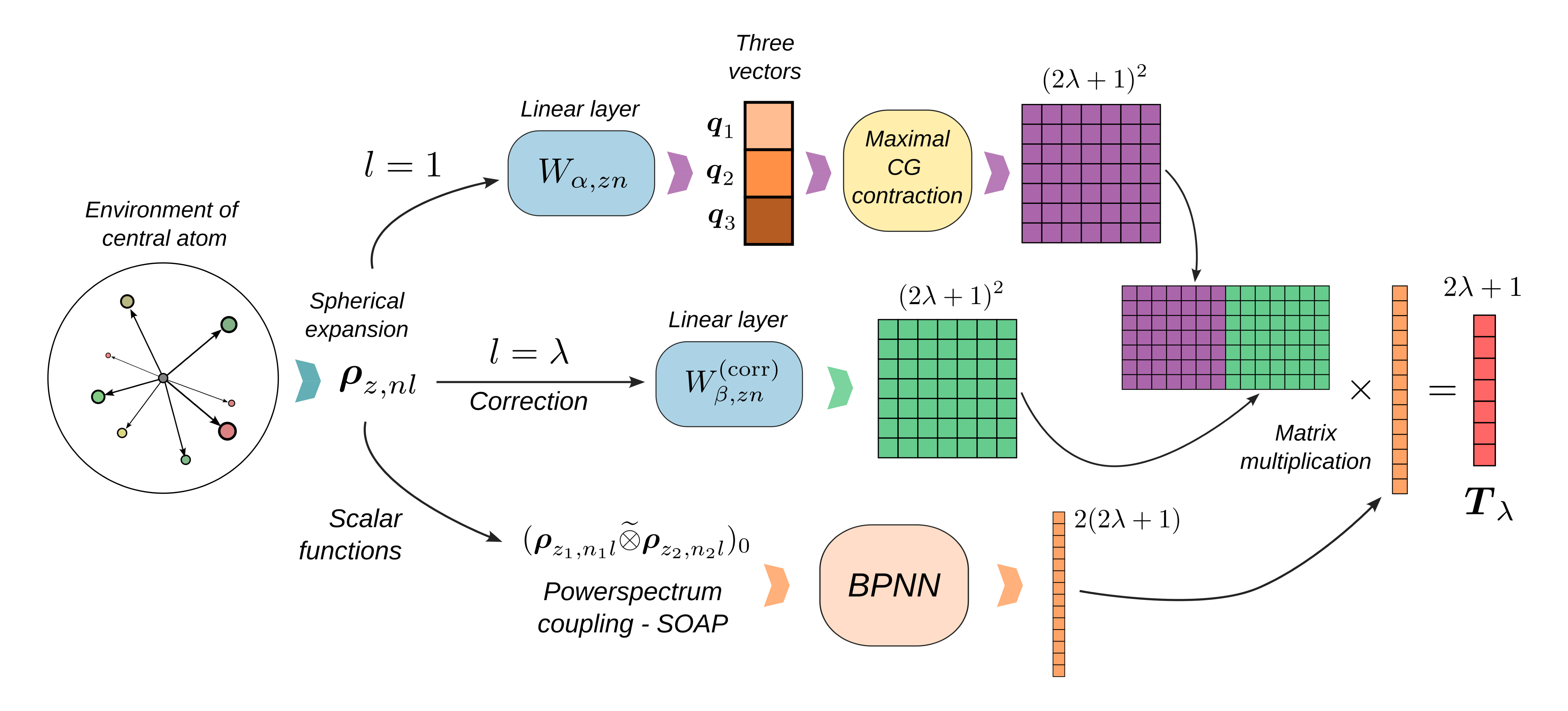
Here is a schematic representation of the \(\lambda\)-MCoV model which, in a nutshell, allows us to learn a tensorial property of a system from a set of scalar features used as linear expansion coefficients of a minimal set of basis tensors.

# visualize a scheme of the architecture that is also used as a thumbnail for the recipe
fig, ax = plt.subplots(figsize=(5728 / 300, 2598 / 300), dpi=300)
img = mpimg.imread("architecture.png")
ax.imshow(img)
ax.axis("off")
fig.tight_layout()
plt.show()

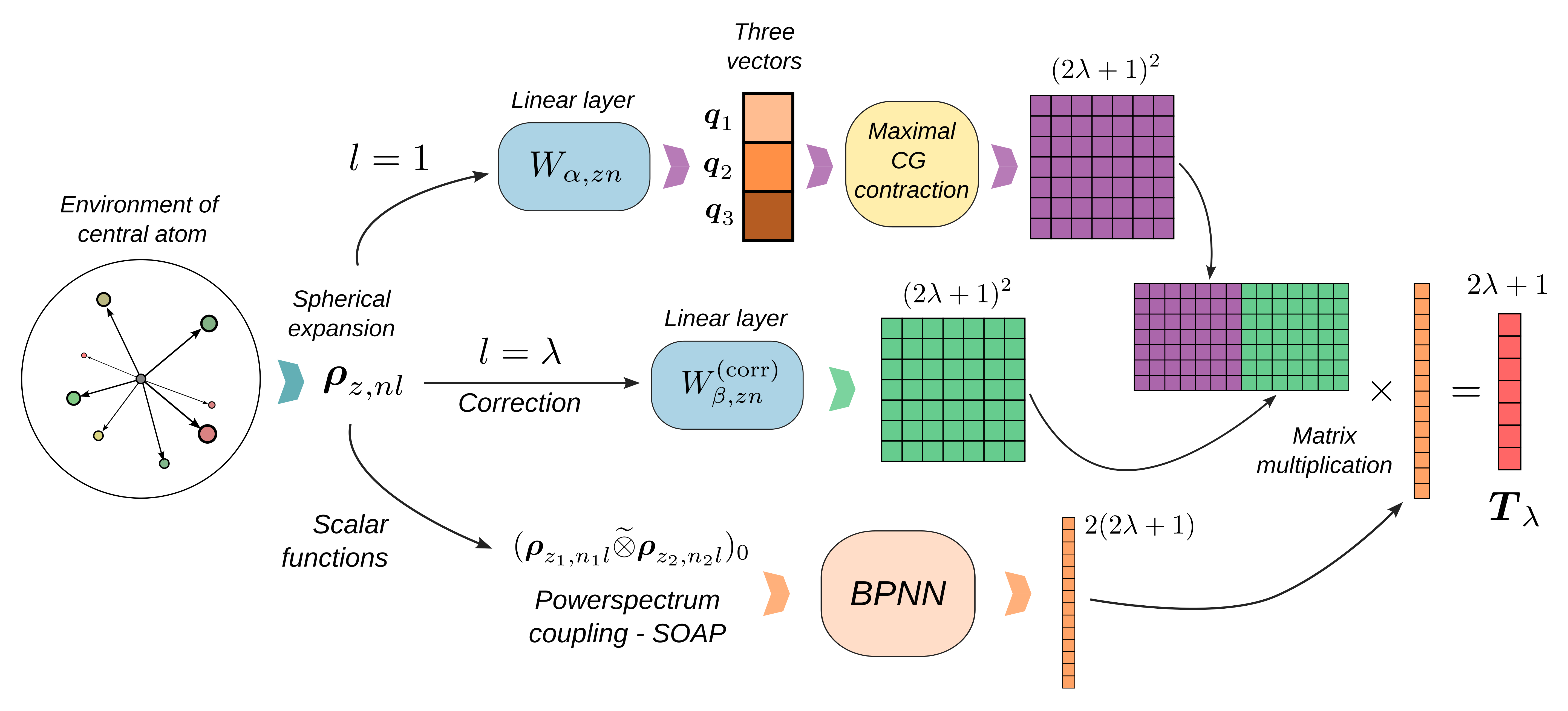
We parametrize spherical tensors of order \(\lambda\) as linear combinations of a small, fixed set of maximally coupled basis tensors. Each basis tensor is computed from three learned vector features, and each coefficient is predicted by a scalar function of the local atomic environment. This enforces exact equivariance under the action of the orthogonal group O(3), while relying only on efficient scalar networks. The architecture is composed as follows:

1. Local Spherical Expansion

We compute atom-centered spherical expansion coefficients of the neighbor density around atom \(i\):

\[\boldsymbol{\rho}_{z,nl} = \sum_{i \in z} R_{n,l}(r_i) \, \boldsymbol{Y}_l(\hat{\mathbf{r}}_i)\]

for orders \(l=1\) (vector basis) up to \(l=\lambda\) (correction).

2. Learned Vector Basis

From the \(l=1\) coefficients, we form three global vectors by a learnable linear layer over species \(z\) and radial channels \(n\):

\[\mathbf{q}_\alpha = \sum_{z,n} W_{\alpha,zn}\,\boldsymbol{\rho}_{z,n1}\]

3. Maximally Coupled Tensor Basis

We build the \(2\lambda+1\) independent components by maximally coupling the three vectors \(\mathbf{q}_1,\mathbf{q}_2,\mathbf{q}_3\). Maximally coupled tensors are defined by contracting their harmonic components to the highest total angular momentum. For example, maximally coupling \(\lambda\) vectors yields:

\[(\underbrace{\mathbf{a}_1 \widetilde{\otimes} \ldots \widetilde{\otimes} \mathbf{a}_\lambda}_{\lambda\text{ times}})_{\lambda\mu} := \Big(\big(\cdots \big((\mathbf{a}_1 \widetilde{\otimes} \mathbf{a}_2)_2 \widetilde{\otimes} \mathbf{a}_3\big)_3\widetilde{\otimes} \cdots \widetilde{\otimes} \mathbf{a}_{\lambda-1}\big)_{\lambda-1}\widetilde{\otimes} \mathbf{a}_\lambda\Big)_{\lambda\mu} \phantom{:}= \sum_{m_1\ldots m_\lambda} \mathcal{C}^{\lambda\mu}_{m_1\ldots m_\lambda}\big((\mathbf{a}_1)_{m_1} \cdot \ldots\cdot (\mathbf{a}_\lambda)_{m_\lambda}\big),\]

where \(\mathcal{C}^{\lambda\mu}_{m_1\ldots m_\lambda}\) a shorthand notation for the components of the tensor \(\mathcal{C}\) obtained by contracting the Clebsch-Gordan coefficients involved in the coupling.

With this definition, vector components can be expressed as

\[\mathbf{T}_{1}(\{\mathbf{r}_i\}) = \sum_{\alpha = 1}^3 f_{\alpha} (\{\mathbf{r}_i\})\,\mathbf{q}_{\alpha},\]

and \(\lambda=2\) components as

\[\begin{split}\mathbf{T}_{2}(\{\mathbf{r}_i\}) = \sum_{\alpha = 1}^2 f_\alpha(\{\mathbf{r}_i\}) \mathbf{q}_\alpha^{\widetilde{\otimes} 2}\,\,+ \sum_{\substack{\alpha_1,\alpha_2= 1\\\alpha_1<\alpha_2}}^{3} g_{\alpha_1\alpha_2}(\{\mathbf{r}_i\}) \big(\mathbf{q}_{\alpha_1}\widetilde{\otimes} \mathbf{q}_{\alpha_2}\big)_{2}.\end{split}\]

More generally, for any \(\lambda>2\) we have:

\[\mathbf{T}_{\lambda} (\{\mathbf{r}_i\}) = \sum_{l= 0}^\lambda f_{l} (\{\mathbf{r}_i\}) \Big(\mathbf{q}_1^{\widetilde{\otimes} l}\widetilde{\otimes} {\mathbf{q}}_2^{\widetilde{\otimes}(\lambda-l)}\Big)_{\lambda}+ \sum_{l=0}^{\lambda-1} g_{l} (\{\mathbf{r}_i\}) \Big(\mathbf{q}^{\widetilde{\otimes} l}_1\widetilde{\otimes} \mathbf{q}_2^{\widetilde{\otimes} (\lambda-l-1)}\widetilde{\otimes} \mathbf{q}_3\Big)_{\lambda\mu}.\]

4. \(\lambda\)-Correction Term

Highly symmetric environments can lead to all-zero vector spherical expansion components, which in turn would yield all-zero tensor features. To correct this, we add a term based on the order \(\lambda\) spherical expansion:

\[\mathbf{T}_\lambda^{\rm corr}(\{\mathbf{r}_i\}) \;=\; \sum_{\beta=1}^{2\lambda+1} h_\beta(\{\mathbf{r}_i\})\, \sum_{z,n}W^{\rm corr}_{\beta,zn}\,\boldsymbol{\rho}_{z,n}^{l=\lambda}\]

with learnable scalar functions \(h_\beta(\{\mathbf{r}_i\})\).

5. Scalar Network (SOAP-BPNN)

We first compute SOAP powerspectrum features:

\[p_{z_1z_2,n_1 n_2,l} = \bigl(\boldsymbol{\rho}_{z_1,n_1 l} \widetilde{\otimes} \boldsymbol{\rho}_{z_2,n_2 l}\bigr)_0\]

and then apply a small, per-species multi-layer perceptron to map these features to scalar coefficients \(f,g,h\).

6. Assembly and Global Output

Finally, we assemble the tensor:

\[\mathbf{T}_\lambda(\{\mathbf{r}_i\}) = \sum_{\beta=1}^{2\lambda+1} s_\beta(\{\mathbf{r}_i\}) \, \mathbf{B}^\lambda_\beta (\mathbf{q}_1,\mathbf{q}_2,\mathbf{q}_3) + \mathbf{T}_\lambda^{\mathrm{corr}} (\{\mathbf{r}_i\}),\]

where \(\mathbf{B}^\lambda_\beta\) is a shorthand for the basis tensors and \(s_\beta\) for the scalar coefficients. For global properties we sum over all atoms.

Training and evaluation of the model

Rather than implementing the \(\lambda\)-MCoV model from scratch, we use a pre-defined architecture within the metatrain package, using its command-line interface. To start training, we run

mtt train options.yaml

The options file specifies the model architecture and the training parameters:

base_precision: 32
seed: 0
architecture:
  name: soap_bpnn
  training:
    batch_size: 10
    num_epochs: 10
    learning_rate: 0.001
    log_interval: 1
training_set:
  systems: 
    read_from: training_set.xyz
  targets: 
    mtt::dipole:
      read_from: training_dipoles.mts
      type: 
        spherical:
          irreps:
            - {o3_lambda: 1, o3_sigma: 1}
    mtt::polarizability:
      read_from: training_polarizabilities.mts
      type: 
        spherical:
          irreps:
            - {o3_lambda: 0, o3_sigma: 1}
            - {o3_lambda: 2, o3_sigma: 1}
validation_set:
  systems: 
    read_from: validation_set.xyz
  targets: 
    mtt::dipole:
      read_from: validation_dipoles.mts
      type: 
        spherical:
          irreps:
            - {o3_lambda: 1, o3_sigma: 1}
    mtt::polarizability:
      read_from: validation_polarizabilities.mts
      type: 
        spherical:
          irreps:
            - {o3_lambda: 0, o3_sigma: 1}
            - {o3_lambda: 2, o3_sigma: 1}
test_set:
  systems: 
    read_from: test_set.xyz
  targets: 
    mtt::dipole:
      read_from: test_dipoles.mts
      type: 
        spherical:
          irreps:
            - {o3_lambda: 1, o3_sigma: 1}
    mtt::polarizability:
      read_from: test_polarizabilities.mts
      type: 
        spherical:
          irreps:
            - {o3_lambda: 0, o3_sigma: 1}
            - {o3_lambda: 2, o3_sigma: 1}

To execute metatrain from within a script, use

subprocess.run(
    [
        "mtt",
        "train",
        "options.yaml",
    ],
    check=True,
)

CompletedProcess(args=['mtt', 'train', 'options.yaml'], returncode=0)

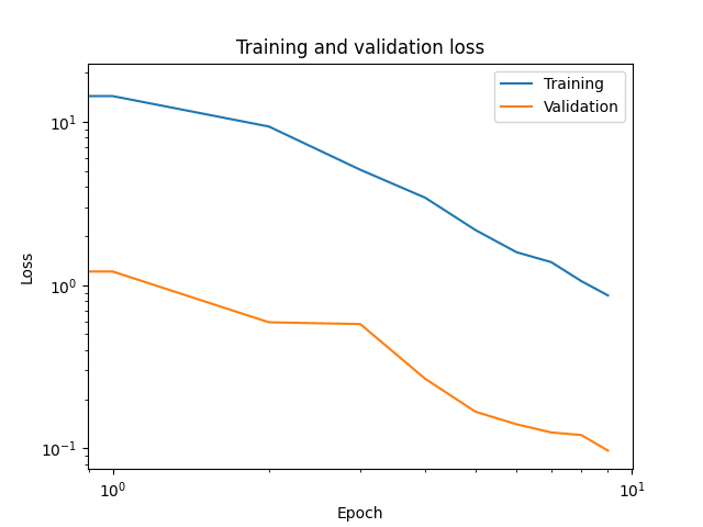
We visualize training and validation losses as functions of the epoch. The training log is stored in CSV format in the outputs directory.

train_log = np.genfromtxt(
    glob("outputs/*/*/train.csv")[-1],
    delimiter=",",
    names=True,
    dtype=None,
    encoding="utf-8",
)[1:]

plt.loglog(train_log["Epoch"], train_log["training_loss"], label="Training")
plt.loglog(train_log["Epoch"], train_log["validation_loss"], label="Validation")
plt.xlabel("Epoch")
plt.ylabel("Loss")
plt.legend()
plt.title("Training and validation loss")

Text(0.5, 1.0, 'Training and validation loss')

We evaluate the model on the test set using the metatrain command-line interface:

mtt eval model.pt eval.yaml -e extensions -o test_results.mts

The evaluation YAML file contains lists the structures and corresponding reference quantities for the evaluation:

systems: 
  read_from: test_set.xyz
targets: 
  mtt::dipole:
    read_from: test_dipoles.mts
    type: 
      spherical:
        irreps:
          - {o3_lambda: 1, o3_sigma: 1}
  mtt::polarizability:
    read_from: test_polarizabilities.mts
    type: 
      spherical:
        irreps:
          - {o3_lambda: 0, o3_sigma: 1}
          - {o3_lambda: 2, o3_sigma: 1}

We can evaluate the model from within the script with

subprocess.run(
    [
        "mtt",
        "eval",
        "model.pt",
        "eval.yaml",
        "-e",
        "extensions",
        "-o",
        "test_results.mts",
    ],
    check=True,
)

CompletedProcess(args=['mtt', 'eval', 'model.pt', 'eval.yaml', '-e', 'extensions', '-o', 'test_results.mts'], returncode=0)

We load the test set predictions and targets from disk and prepare them for comparison. Predictions are in test_results_mtt::dipole.mts and test_results_mtt::polarizability.mts. Targets are in test_dipoles.mts and test_polarizabilities.mts. We can load them using the metatensor.load() function.

prediction_test = {
    "dipole": mts.load("test_results_mtt::dipole.mts"),
    "polarizability": mts.load("test_results_mtt::polarizability.mts"),
}

target_test = {
    "dipole": mts.load("test_dipoles.mts"),
    "polarizability": mts.load("test_polarizabilities.mts"),
}

test_set_molecules = ase.io.read("test_set.xyz", ":")
natm = np.array([len(mol) for mol in test_set_molecules])

We create parity plots comparing predicted and target values for each target quantity and for each \(\lambda\) component.

color_per_lambda = {0: "C0", 1: "C1", 2: "C2"}

fig, axes = plt.subplots(1, 2)
for ax, key in zip(axes, prediction_test):

    ax.set_aspect("equal")

    pred = prediction_test[key]
    target = target_test[key]

    for k in target.keys:
        assert k in pred.keys
        o3_lambda = int(k["o3_lambda"])
        label = rf"$\lambda={o3_lambda}$"
        x = target[k].values[..., 0] / natm[:, np.newaxis]
        y = pred[k].values[..., 0] / natm[:, np.newaxis]
        ax.plot(
            x.flatten(),
            y.flatten(),
            ".",
            color=color_per_lambda[o3_lambda],
            label=label,
        )

    xmin, xmax = ax.get_xlim()
    ax.plot([xmin, xmax], [xmin, xmax], "k--", lw=1)
    ax.set_xlim(xmin, xmax)
    ax.set_ylim(xmin, xmax)

    ax.set_xlabel("Target (a.u./atom)")
    ax.set_ylabel("Prediction (a.u./atom)")

    ax.set_title(key.capitalize())

    ax.legend()
fig.tight_layout()