MD using direct-force predictions with PET-MAD

Authors:

Michele Ceriotti @ceriottm, Filippo Bigi @frostedoyster

Evaluating forces as a direct output of a ML model accelerates their evaluation, by up to a factor of 3 in comparison to the traditional approach that evaluates them as derivatives of the interatomic potential. Unfortunately, as discussed e.g. in this preprint, doing so means that forces are not conservative, leading to instabilities and artefacts in many modeling tasks, such as constant-energy molecular dynamics. Here we demonstrate the issues associated with direct force predictions, and ways to mitigate them, using the generally-applicable PET-MAD potential. See also this recipe for examples of using PET-MAD for basic tasks such as geometry optimization and conservative MD.

# sphinx_gallery_thumbnail_number = 2

If you don’t want to use the conda environment for this recipe, you can get all dependencies installing the PET-MAD package:

pip install pet-mad

import os
import time

import ase.io

# i-PI scripting utilities
import chemiscope
import matplotlib.pyplot as plt
import metatensor.torch.atomistic as mta
from ipi.utils.parsing import read_output, read_trajectory
from ipi.utils.scripting import InteractiveSimulation

# pet-mad ASE calculator
from pet_mad.calculator import PETMADCalculator


if hasattr(__import__("builtins"), "get_ipython"):
    get_ipython().run_line_magic("matplotlib", "inline")  # noqa: F821

Fetch PET-MAD and export the model

We first download the latest version of the PET-MAD model, and export the model as a torchscript file.

# downloads the model checkpoint and export it
model_filename = "pet-mad-latest.pt"
if not os.path.exists(model_filename):
    calculator = PETMADCalculator(version="latest", device="cpu")
    calculator.model.save(model_filename)

The model can also be loaded from this torchscript dump, which often speeds up calculation as it involves compilation, and is functionally equivalent unless you plan on fine-tuning, or otherwise modifying the model.

calculator = mta.ase_calculator.MetatensorCalculator(model_filename, device="cpu")

Non-conservative forces

Interatomic potentials are typically used to compute the forces acting on the atoms by differentiating with respect to atomic positions, i.e. if

\[V(\mathbf{r}_1, \mathbf{r}_2, \ldots \mathbf{r}_n)\]

is the potential for an atomic configuration then the force acting on atom \(i\) is

\[\mathbf{f}_i = \partial V/\partial \mathbf{r}_i\]

Even though the early ML-based interatomic potentials followed this route, computing forces directly as a function of the atomic coordinates, as additional heads of the same model that computes \(V\), is computationally more efficient (between 2x and 3x faster). The MetatensorCalculator class allows one to choose between conservative (back-propagated) and non-conservative (direct) force evaluation

structure = ase.io.read("data/bmimcl.xyz")

structure.calc = calculator
energy_c = structure.get_potential_energy()
forces_c = structure.get_forces()

calculator_nc = mta.ase_calculator.MetatensorCalculator(
    model_filename, device="cpu", non_conservative=True
)

structure.calc = calculator_nc
energy_nc = structure.get_potential_energy()
# forces_nc = structure.get_forces() # temporarily broken

print(f"Energy:\n  Conservative: {energy_c:.8}\n  Non-conserv.: {energy_nc:.8}")

Energy:
  Conservative: -2378.8296
  Non-conserv.: -2378.8296

Energy conservation in NVE molecular dynamics

Molecular dynamics simply integrates Hamilton’s equations

\[\dot{\mathbf{r}}_i = \mathbf{p}_i/m_i \quad \dot{\mathbf{p}}_i = \mathbf{f}_i\]

to evolve in time the atomic positions. When the forces are the derivatives of a potential energy \(V\), these equations conserve the total energy \(H = V+\sum_i\mathbf{p}_i^2/2m_i\).

Finite time step integrators only conserve energy approximately, but usually stable dynamics implies a high level of conservation, and no long-time drift. Here we demonstrate the impact of direct force prediction on energy conservation, using a short MD trajectory of 1-Butyl-3-methylimidazolium chloride (BMIM-Cl).

Conservative forces

First, we run a few steps computing forces as derivatives of the potential. The MD setup is described in the input-nve.xml file. This is a rather standard setup, with the key parameters being those given in the <ffdirect> section.

with open("data/input-nve.xml", "r") as file:
    input_nve = file.read()
print(input_nve)

<simulation verbosity="low">
<output prefix="nve-c">
    <properties stride="8" filename="out">
                [step, time{picosecond}, conserved{electronvolt}, temperature{kelvin},
        kinetic_md{electronvolt}, potential{electronvolt},
        pot_component(0){electronvolt}
                ]
    </properties>
    <trajectory filename="pos" stride="16" format="ase"> positions </trajectory>
    <trajectory filename="forces_c" stride="16" format="ase"> forces_component(0) </trajectory>
    <checkpoint stride="1000"/>
</output>
<total_steps>32</total_steps>
<prng><seed>12345</seed></prng>
<ffdirect  name='cons' pbc="false">
    <pes>metatensor</pes>
    <parameters>{template:data/bmimcl.xyz,model:pet-mad-latest.pt,device:cpu,non_conservative:False} </parameters>
</ffdirect>
<system>
    <initialize nbeads="1">
        <file mode="ase"> data/bmimcl.xyz </file>
        <velocities mode="thermal" units="kelvin"> 400.0 </velocities>
    </initialize>
    <forces>
        <force forcefield="cons">
        </force>
    </forces>

    <motion mode="dynamics">
        <dynamics mode="nve">
                <timestep units="femtosecond"> 0.5 </timestep>
        </dynamics>
    </motion>

</system>
</simulation>

The simulation can also be run from the command line using

i-pi data/input-nve.xml

but here we run interactively, timing the execution for comparison.

sim = InteractiveSimulation(input_nve)
steps_nve_c = 32
time_nve_c = -time.time()
sim.run(steps_nve_c)
time_nve_c += time.time()
time_nve_c /= steps_nve_c + 1  # there's one extra energy evaluation at the beginning

 @system: Initializing system object
 @simulation: Initializing simulation object
@ RANDOM SEED: The seed used in this calculation was 12345
 @init_file: Initializing from file data/bmimcl.xyz. Dimension: length, units: automatic, cell_units: automatic
 @init_file: Initializing from file data/bmimcl.xyz. Dimension: length, units: automatic, cell_units: automatic
 @init_file: Initializing from file data/bmimcl.xyz. Dimension: length, units: automatic, cell_units: automatic
 @init_file: Initializing from file data/bmimcl.xyz. Dimension: length, units: automatic, cell_units: automatic
 @init_file: Initializing from file data/bmimcl.xyz. Dimension: length, units: automatic, cell_units: automatic
 @initializer: Resampling velocities at temperature 400.0 kelvin
 @system.bind: Binding the forces
 @simulation.run: Average timings at MD step       0. t/step: 2.88640e+00

Non-conservative (direct) forces

The PET-MAD model provides direct force predictions, that can be activated with a non_conservative:True flag. This makes it very simple to modify the NVE setup:

with open("data/input-nc-nve.xml", "r") as file:
    input_nve = file.read()
print(input_nve[574:764])

<ffdirect  name='nocons' pbc="false">
    <pes>metatensor</pes>
    <parameters>{template:data/bmimcl.xyz,model:pet-mad-latest.pt,device:cpu,non_conservative:True} </parameters>
</ffdirect>

We run this example for longer (it is faster!) and time it for comparison

sim = InteractiveSimulation(input_nve)
steps_nve_nc = 128
time_nve_nc = -time.time()
sim.run(steps_nve_nc)
time_nve_nc += time.time()
time_nve_nc /= steps_nve_nc + 1

 @system: Initializing system object
 @simulation: Initializing simulation object
@ RANDOM SEED: The seed used in this calculation was 12345
 @init_file: Initializing from file data/bmimcl.xyz. Dimension: length, units: automatic, cell_units: automatic
 @init_file: Initializing from file data/bmimcl.xyz. Dimension: length, units: automatic, cell_units: automatic
 @init_file: Initializing from file data/bmimcl.xyz. Dimension: length, units: automatic, cell_units: automatic
 @init_file: Initializing from file data/bmimcl.xyz. Dimension: length, units: automatic, cell_units: automatic
 @init_file: Initializing from file data/bmimcl.xyz. Dimension: length, units: automatic, cell_units: automatic
 @initializer: Resampling velocities at temperature 400.0 kelvin
 @system.bind: Binding the forces
 @simulation.run: Average timings at MD step       0. t/step: 1.35456e+00
 @open_backup: Backup performed: RESTART -> #RESTART#0#

The simulation generates output files that can be parsed and visualized from Python.

data_c, info = read_output("nve-c.out")
data_nc, info = read_output("nve-nc.out")

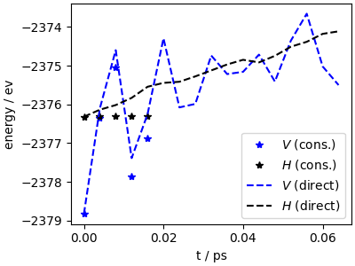
There is a large drift of the onserved quantity, that is also associated in a rapid increase of the potential energy, which indicates that the lack of conservative behavior distorts the sampled ensemble (and in fact, would lead to loss of structural integrity in a longer run).

fig, ax = plt.subplots(1, 1, figsize=(4, 3), constrained_layout=True)

ax.set_facecolor("white")
ax.plot(data_c["time"], data_c["potential"], "b*", label=r"$V$ (cons.)")
ax.plot(data_c["time"], data_c["conserved"] - 20, "k*", label=r"$H$ (cons.)")
ax.plot(data_nc["time"], data_nc["potential"], "b--", label=r"$V$ (direct)")
ax.plot(data_nc["time"], data_nc["conserved"] - 20, "k--", label=r"$H$ (direct)")
ax.set_xlabel("t / ps")
ax.set_ylabel("energy / ev")
ax.legend()

<matplotlib.legend.Legend object at 0x7f18641c60f0>

Energy conservation at low-cost with multiple time stepping

Given that PET-MAD provides both direct and conservative forces, it is possible to implement a simulation strategy that achieves a high degree of energy conservation at a cost that is close to that of direct-force MD. This relies on the multiple time stepping (MTS) idea, which is discussed and demonstrated in this recipe.

The key idea is to perform several steps of MD using the short timestep needed to follow atomic motion, and a “cheap” force evaluator \(\mathbf{f}_{\mathrm{fast}}\), and then apply a correction \(\mathbf{f}_{\mathrm{slow}}\) every \(M\) of such steps. In this case, the fast forces are the direct predictions, and the slow ones the difference between conservative and direct forces.

This simulation setup can be realized readily in i-PI.

with open("data/input-nc-nve-mts.xml", "r") as file:
    input_nve_mts = file.read()

First, one can define two forcefields that compute conservative and direct forces

print(input_nve_mts[704:1082])

<ffdirect  name='cons' pbc="false">
    <pes>metatensor</pes>
    <parameters>{template:data/bmimcl.xyz,model:pet-mad-latest.pt,device:cpu,non_conservative:False} </parameters>
</ffdirect>
<ffdirect  name='nocons' pbc="false">
    <pes>metatensor</pes>
    <parameters>{template:data/bmimcl.xyz,model:pet-mad-latest.pt,device:cpu,non_conservative:True} </parameters>
</ffdirect>

… then, use them in the definition of the systems, specifying how to weight them at each MTS level

print(input_nve_mts[1258:1482])

<forces>
    <force forcefield="cons">
        <mts_weights>[1,0]</mts_weights>
    </force>
    <force forcefield="nocons">
        <mts_weights>[-1,1]</mts_weights>
    </force>
</forces>

… and finally request the appropriate MTS discretization in the integrator: this specifies that the inner loop should be executed 8 times, and the outer loop (which has an overall time step of 4 fs) once per step

print(input_nve_mts[1480:1655])

<motion mode="dynamics">
    <dynamics mode="nve">
            <timestep units="femtosecond"> 4 </timestep>
        <nmts>[1,8]</nmts>
    </dynamics>
</motion>

All of this happens behind the scenes, and the simulation is just run as for the simpler MD cases. Note also that it is possible to combine this with thermostatted or NPT dynamics, in a completely seamless manner

sim = InteractiveSimulation(input_nve_mts)
nmts = 8
steps_nve_mts = steps_nve_nc // nmts
time_nve_mts = -time.time()
sim.run(steps_nve_mts)
time_nve_mts += time.time()
time_nve_mts /= steps_nve_mts * nmts + 1

 @system: Initializing system object
 @simulation: Initializing simulation object
@ RANDOM SEED: The seed used in this calculation was 12345
 @init_file: Initializing from file data/bmimcl.xyz. Dimension: length, units: automatic, cell_units: automatic
 @init_file: Initializing from file data/bmimcl.xyz. Dimension: length, units: automatic, cell_units: automatic
 @init_file: Initializing from file data/bmimcl.xyz. Dimension: length, units: automatic, cell_units: automatic
 @init_file: Initializing from file data/bmimcl.xyz. Dimension: length, units: automatic, cell_units: automatic
 @init_file: Initializing from file data/bmimcl.xyz. Dimension: length, units: automatic, cell_units: automatic
 @initializer: Resampling velocities at temperature 400.0 kelvin
 @system.bind: Binding the forces
 @simulation.run: Average timings at MD step       0. t/step: 1.08573e+01
 @open_backup: Backup performed: RESTART -> #RESTART#1#

The MTS calculation recovers most of the speedup of direct forces

print(
    f"""
Time per 0.5fs step:
Conservative forces: {time_nve_c:.4f} s/step
Direct forces:       {time_nve_nc:.4f} s/step
MTS (M=8):           {time_nve_mts:.4f} s/step
"""
)

Time per 0.5fs step:
Conservative forces: 2.4106 s/step
Direct forces:       0.9526 s/step
MTS (M=8):           1.2299 s/step

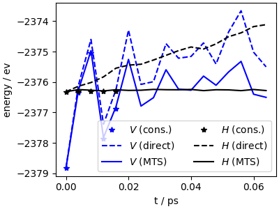
… and the energy conservation is on par with the conservative trajectory (although the actual trajectories would deviate from each other due to accumulation of small errors, but the overall sampling is reliable on a long timescale).

data_mts, info = read_output("nve-nc-mts.out")
trj_mts = read_trajectory("nve-nc-mts.pos_0.extxyz")
force_c_mts = read_trajectory("nve-nc-mts.forces_c.extxyz")
force_nc_mts = read_trajectory("nve-nc-mts.forces_nc.extxyz")
#

fig, ax = plt.subplots(1, 1, figsize=(4, 3), constrained_layout=True)

ax.set_facecolor("white")
ax.plot(data_c["time"], data_c["potential"], "b*", label=r"$V$ (cons.)")
ax.plot(data_nc["time"], data_nc["potential"], "b--", label=r"$V$ (direct)")
ax.plot(data_mts["time"], data_mts["potential"], "b-", label=r"$V$ (MTS)")
ax.plot(data_c["time"], data_c["conserved"] - 20, "k*", label=r"$H$ (cons.)")
ax.plot(data_nc["time"], data_nc["conserved"] - 20, "k--", label=r"$H$ (direct)")
ax.plot(data_mts["time"], data_mts["conserved"] - 20, "k-", label=r"$H$ (MTS)")
ax.set_xlabel("t / ps")
ax.set_ylabel("energy / ev")
ax.legend(ncols=2)

<matplotlib.legend.Legend object at 0x7f1851ff4e60>

i-PI prints out both force components for diagnostics, which we can visualize along the (short) trajectory. The conservative forces are shown in atom colors, and the direct predictions in red. One sees clearly that the two predictions are quite close, so the correction is small and can be successfully applied with a large MTS stride.

cs_forces_c = chemiscope.ase_vectors_to_arrows(
    force_c_mts, "forces_component", scale=1.0
)
cs_forces_nc = chemiscope.ase_vectors_to_arrows(
    force_nc_mts, "forces_component", scale=1.0
)
cs_forces_nc["parameters"]["global"]["color"] = "#aa0000"

chemiscope.show(
    trj_mts,
    mode="default",
    properties={
        "time": data_mts["time"][::2],
        "conserved": data_mts["conserved"][::2],
        "potential": data_mts["potential"][::2],
    },
    shapes={
        "forces_c": cs_forces_c,
        "forces_nc": cs_forces_nc,
    },
    settings=chemiscope.quick_settings(
        x="time",
        y="potential",
        structure_settings={"unitCell": True, "shape": ["forces_c", "forces_nc"]},
        trajectory=True,
    ),
)

×