Equivariant linear model for polarizability

Authors:

Paolo Pegolo @ppegolo

In this example, we demonstrate how to construct a metatensor atomistic model for the polarizability tensor of molecular systems. This example uses the featomic library to compute equivariant descriptors, and scikit-learn to train a linear regression model. The model can then be used in an ASE calculator.

from typing import Dict, List, Optional

import ase.io
import chemiscope

# Simulation and visualization tools
import matplotlib.pyplot as plt
import metatensor.torch as mts

# Model wrapping and execution tools
import numpy as np
import torch
from featomic.torch import SphericalExpansion
from featomic.torch.clebsch_gordan import (
    EquivariantPowerSpectrum,
    cartesian_to_spherical,
)
from metatensor.torch import Labels, TensorBlock, TensorMap
from metatensor.torch.atomistic import (
    MetatensorAtomisticModel,
    ModelCapabilities,
    ModelEvaluationOptions,
    ModelMetadata,
    ModelOutput,
    System,
    load_atomistic_model,
    systems_to_torch,
)
from metatensor.torch.atomistic.ase_calculator import MetatensorCalculator
from metatensor.torch.learn.nn import EquivariantLinear

# Core libraries
from sklearn.linear_model import RidgeCV


torch.set_default_dtype(torch.float64)  # FIXME: This is a temporary fix

if hasattr(__import__("builtins"), "get_ipython"):
    get_ipython().run_line_magic("matplotlib", "inline")  # noqa: F821

Polarizability tensor

The polarizability tensor describes the response of a molecule to an external electric field.

\[\alpha_{ij} = \frac{\partial^2 U}{\partial E_i \partial E_j}\]

It is a rank-2 symmetric tensor and it can be decomposed into irreducible spherical components. Due to its symmetry, only the components with \(\lambda=0\) and \(\lambda=2\) are non-zero. The \(\lambda=0\) component is a scalar, while the \(\lambda=2\) component corresponds to a symmetric traceless matrix

Load the training data

We load a simple dataset of \(\mathrm{C}_5\mathrm{NH}_7\) molecules and their polarizability tensors stored in extended XYZ format. We also visualize the polarizability as ellipsoids to demonstrate the anisotropy of this molecular property.

ase_frames = ase.io.read("data/qm7x_reduced_100.xyz", index=":")

ellipsoids = chemiscope.ase_tensors_to_ellipsoids(
    ase_frames, "polarizability", scale=0.15
)
ellipsoids["parameters"]["global"]["color"] = "#FF8800"
cs = chemiscope.show(
    ase_frames,
    shapes={"alpha": ellipsoids},
    mode="structure",
    settings=chemiscope.quick_settings(
        structure_settings={"shape": ["alpha"]}, trajectory=True
    ),
)
cs

×

Read the polarizability tensors and store them in a TensorMap

We extract the polarizability tensors from the extended XYZ file and store them in a metatensor.torch.TensorMap. The polarizability tensors are stored as Cartesian tensors.

cartesian_polarizability = np.stack(
    [frame.info["polarizability"].reshape(3, 3) for frame in ase_frames]
)
cartesian_tensormap = TensorMap(
    keys=Labels.single(),
    blocks=[
        TensorBlock(
            samples=Labels.range("system", len(ase_frames)),
            components=[Labels.range(name, 3) for name in ["xyz_1", "xyz_2"]],
            properties=Labels(["polarizability"], torch.tensor([[0]])),
            values=torch.from_numpy(cartesian_polarizability).unsqueeze(-1),
        )
    ],
)

print(cartesian_tensormap)
print(cartesian_tensormap.block(0))

TensorMap with 1 blocks
keys: _
      0
TensorBlock
    samples (100): ['system']
    components (3, 3): ['xyz_1', 'xyz_2']
    properties (1): ['polarizability']
    gradients: None

We also convert the Cartesian tensors to irreducible spherical tensors using the featomic.torch.clebsch_gordan.cartesian_to_spherical() function. Now the polarizability is stored in a metatensor.torch.TensorMap object that contains two metatensor.torch.TensorBlock labeled by the irreducible spherical components as keys.

spherical_tensormap = mts.remove_dimension(
    cartesian_to_spherical(cartesian_tensormap, components=["xyz_1", "xyz_2"]),
    "keys",
    "_",
)

print(spherical_tensormap)
print(spherical_tensormap.block(0))
print(spherical_tensormap.block(1))

TensorMap with 2 blocks
keys: o3_lambda  o3_sigma
          0         1
          2         1
TensorBlock
    samples (100): ['system']
    components (1): ['o3_mu']
    properties (1): ['polarizability']
    gradients: None

TensorBlock
    samples (100): ['system']
    components (5): ['o3_mu']
    properties (1): ['polarizability']
    gradients: None

Split the dataset

The dataset is split into training and test sets using a 80/20 ratio. We also visualize the polarizability as ellipsoids to e into training and test sets according to the indices previously defined.

n_frames = len(ase_frames)
train_idx = np.random.choice(n_frames, int(0.8 * n_frames), replace=False)
test_idx = np.setdiff1d(np.arange(n_frames), train_idx)
spherical_tensormap_train = mts.slice(
    spherical_tensormap,
    "samples",
    Labels("system", torch.from_numpy(train_idx).reshape(-1, 1)),
)
cartesian_tensormap_test = mts.slice(
    cartesian_tensormap,
    "samples",
    Labels("system", torch.from_numpy(test_idx).reshape(-1, 1)),
)

Equivariant model for polarizability

The polarizability tensor can be predicted using equivariant linear models. In this example, we use the featomic library to compute equivariant \(\lambda\)-SOAP descriptors, adapted to the symmetry of the irreducible components of \(\boldsymbol{\alpha}\) and scikit-learn to train a symmetry-adapted linear ridge regression model.

Utility functions

We define a couple of utility functions to convert the spherical polarizability tensor back to a Cartesian tensor.

The first utility function takes the \(\lambda=2\) spherical components and reconstructs the \(3 \times 3\) symmetric traceless matrix.

def matrix_from_l2_components(l2: torch.Tensor) -> torch.Tensor:
    """
    Inverts the spherical projection function for a symmetric, traceless 3x3 tensor.

    Given:
        l2 : array-like of 5 components
            These are the irreducible spherical components multiplied by sqrt(2),
            i.e., l2 = sqrt(2) * [t0, t1, t2, t3, t4], where:
                t0 = (A[0,1] + A[1,0])/2
                t1 = (A[1,2] + A[2,1])/2
                t2 = (2*A[2,2] - A[0,0] - A[1,1])/(2*sqrt(3))
                t3 = (A[0,2] + A[2,0])/2
                t4 = (A[0,0] - A[1,1])/2

    Returns:
        A : (3,3) numpy array
            The symmetric, traceless matrix reconstructed from the components.
    """
    # Recover the t_i by dividing by sqrt(2)
    sqrt2 = torch.sqrt(torch.tensor(2.0, dtype=l2.dtype))
    sqrt3 = torch.sqrt(torch.tensor(3.0, dtype=l2.dtype))
    l2 = l2 / sqrt2

    # Allocate the 3x3 matrix A
    A = torch.empty((3, 3), dtype=l2.dtype)

    # Diagonal entries:
    # Use the traceless condition A[0,0] + A[1,1] + A[2,2] = 0.
    # Also, from the definitions:
    #   t4 = (A[0,0] - A[1,1]) / 2
    #   t2 = (2*A[2,2] - A[0,0] - A[1,1])/(2*sqrt3)
    #
    # Solve for A[0,0] and A[1,1]:
    A[0, 0] = -(sqrt3 * l2[2]) / 3 + l2[4]
    A[1, 1] = -(sqrt3 * l2[2]) / 3 - l2[4]
    A[2, 2] = (2 * sqrt3 * l2[2]) / 3  # Since A[2,2] = - (A[0,0] + A[1,1])

    # Off-diagonals:
    A[0, 1] = l2[0]
    A[1, 0] = l2[0]

    A[1, 2] = l2[1]
    A[2, 1] = l2[1]

    A[0, 2] = l2[3]
    A[2, 0] = l2[3]

    return A

The second utility function takes the spherical polarizability tensor and uses the matrix_from_l2_components function to reconstruct symmetric traceless part of the Cartesian tensor, and then combines it with the scalar part to reconstruct the full Cartesian tensor.

def spherical_to_cartesian(spherical_tensor: TensorMap) -> TensorMap:

    dtype = spherical_tensor[0].values.dtype

    new_block: Dict[int, torch.Tensor] = {}

    eye = torch.eye(3, dtype=dtype)
    sqrt3 = torch.sqrt(torch.tensor(3.0, dtype=dtype))
    block_0 = spherical_tensor[0]
    block_2 = spherical_tensor[1]
    system_ids = block_0.samples.values.flatten()

    for i, A in enumerate(system_ids):
        new_block[int(A)] = -block_0.values[
            i
        ].flatten() * eye / sqrt3 + matrix_from_l2_components(
            block_2.values[i].squeeze()
        )

    return TensorMap(
        keys=Labels(["_"], torch.tensor([[0]], dtype=torch.int32)),
        blocks=[
            TensorBlock(
                samples=Labels(
                    "system",
                    torch.tensor(
                        [k for k in new_block.keys()], dtype=torch.int32
                    ).reshape(-1, 1),
                ),
                components=[
                    Labels(
                        "xyz_1",
                        torch.tensor([0, 1, 2], dtype=torch.int32).reshape(-1, 1),
                    ),
                    Labels(
                        "xyz_2",
                        torch.tensor([0, 1, 2], dtype=torch.int32).reshape(-1, 1),
                    ),
                ],
                properties=Labels(["_"], torch.tensor([[0]], dtype=torch.int32)),
                values=torch.stack(
                    [new_block[A] for A in new_block]
                ).unsqueeze(  # .roll((-1, -1), dims=(1, 2))
                    -1
                ),
            )
        ],
    )

Implementation of a torch module for polarizability

In order to implement a polarizability model compatible with metatomic, we need to we need to define a torch.nn.Module with a forward method that takes a list of metatensor.torch.atomistic.System and returns a dictionary of metatensor.torch.TensorMap objects. The forward method must be compatible with TorchScript.

Here, the PolarizabilityModel class is defined. It takes as input a SphericalExpansion object, a list of atomic types, and dtype. The forward method computes the descriptors and applies the linear model to predict the polarizability tensor.

class PolarizabilityModel(torch.nn.Module):
    def __init__(
        self,
        spex_calculator: SphericalExpansion,
        atomic_types: List[int],
        dtype: torch.dtype = None,
    ) -> None:

        super().__init__()

        if dtype is None:
            dtype = torch.float64
        self.dtype = dtype
        device = torch.device("cpu")

        self.hypers = spex_calculator.parameters

        # Check that the atomic types are unique
        assert len(set(atomic_types)) == len(atomic_types)
        self.atomic_types = atomic_types

        # Define lambda soap calculator
        self.lambda_soap_calculator = EquivariantPowerSpectrum(
            spex_calculator, dtype=self.dtype
        )
        self.selected_keys = mts.Labels(
            ["o3_lambda", "o3_sigma"], torch.tensor([[0, 1], [2, 1]])
        )
        self._compute_metadata()

        # Define the linear model that wraps the ridge regression results
        in_keys = self.metadata.keys
        in_features = [block.values.shape[-1] for block in self.metadata]
        out_features = [1 for _ in self.metadata]
        out_properties = [mts.Labels.single() for _ in self.metadata]

        self.linear_model = EquivariantLinear(
            in_keys=in_keys,
            in_features=in_features,
            out_features=out_features,
            out_properties=out_properties,
            dtype=self.dtype,
            device=device,
        )

    def fit(self, training_systems, training_targets, alphas=None):

        lambda_soap = self._compute_descriptor(training_systems)

        ridges: List[RidgeCV] = []
        for k in lambda_soap.keys:
            X = lambda_soap.block(k).values
            y = training_targets.block(k).values
            n_samples, n_components, n_properties = X.shape
            X = X.reshape(n_samples * n_components, n_properties)
            y = y.reshape(n_samples * n_components, -1)
            ridge = RidgeCV(alphas=alphas, fit_intercept=int(k["o3_lambda"]) == 0)
            ridge.fit(X, y)
            ridges.append(ridge)

        self._apply_weights(ridges)

    def _compute_metadata(self):
        # Create dummy system to get the property dimension
        dummy_system = systems_to_torch(
            ase.Atoms(
                numbers=self.atomic_types,
                positions=[[i / 4, 0, 0] for i in range(len(self.atomic_types))],
            )
        )

        self.metadata = self.lambda_soap_calculator.compute_metadata(
            dummy_system, selected_keys=self.selected_keys, neighbors_to_properties=True
        ).keys_to_samples("center_type")

    def _apply_weights(self, ridges: List[RidgeCV]) -> None:
        with torch.no_grad():
            for model, ridge in zip(self.linear_model.module_map, ridges):
                model.weight.copy_(torch.tensor(ridge.coef_, dtype=self.dtype))
                if model.bias is not None:
                    model.bias.copy_(torch.tensor(ridge.intercept_, dtype=self.dtype))

    def _compute_descriptor(self, systems: List[System]) -> TensorMap:
        # Actually compute lambda-SOAP power spectrum
        lambda_soap = self.lambda_soap_calculator(
            systems,
            selected_keys=self.selected_keys,
            neighbors_to_properties=True,
        )

        # Move the `center_type` keys to the sample dimension
        lambda_soap = lambda_soap.keys_to_samples("center_type")

        # Polarizability is a "per-structure" quantity. We don't need to keep
        # `center_type` and `atom` in samples, as we only need to predict the
        # polarizability of the whole structure.
        # A simple way to do so, is summing the descriptors over the `center_type` and
        # `atom` sample dimensions.
        lambda_soap = mts.sum_over_samples(lambda_soap, ["center_type", "atom"])

        return lambda_soap

    def forward(
        self,
        systems: List[System],  # noqa
        outputs: Dict[str, ModelOutput],  # noqa
        selected_atoms: Optional[Labels] = None,  # noqa
    ) -> Dict[str, TensorMap]:  # noqa

        if list(outputs.keys()) != ["cookbook::polarizability"]:
            raise ValueError(
                f"`outputs` keys ({', '.join(outputs.keys())}) contain unsupported "
                "keys. Only 'cookbook::polarizability' is supported."
            )

        if outputs["cookbook::polarizability"].per_atom:
            raise NotImplementedError("per-atom polarizabilities are not supported.")

        # Compute the descriptors
        lambda_soap = self._compute_descriptor(systems)

        # Apply the linear model
        prediction = self.linear_model(lambda_soap)
        prediction = spherical_to_cartesian(prediction)
        # fails at saving due to TorchScript
        return {"cookbook::polarizability": prediction}

Train the polarizability model

We train the polarizability model using the training data. We need to define the hyperparameters for the featomic.torch.SphericalExpansion calculator and the atomic types in the dataset to initialize the module.

hypers = {
    "cutoff": {"radius": 4.5, "smoothing": {"type": "ShiftedCosine", "width": 0.1}},
    "density": {"type": "Gaussian", "width": 0.3},
    "basis": {
        "type": "TensorProduct",
        "max_angular": 3,
        "radial": {"type": "Gto", "max_radial": 3},
    },
}
atomic_types = np.unique(
    np.concatenate([frame.numbers for frame in ase_frames])
).tolist()

spherical_expansion_calculator = SphericalExpansion(**hypers)

Convert ASE frames to metatensor.atomistic.System objects.

Instantiate the polarizability model.

model = PolarizabilityModel(
    spherical_expansion_calculator,
    atomic_types,
    dtype=torch.float64,
)

The ridge regression is performed as with a scikit-learn-style fit method, and the resulting weights are then used to initialize a metatensor.learn.nn.EquivariantLinear module. The PolariabilityModel.fit() method takes the training systems in metatensor.torch.atomistic.System format and the training target metatensor.torch.TensorMap as input. The alphas parameter is used to specify the range of regularization parameters to be tested.

systems_train = [
    system.to(dtype=torch.float64)
    for system in systems_to_torch([ase_frames[i] for i in train_idx])
]
alphas = np.logspace(-6, 6, 50)

model.fit(systems_train, spherical_tensormap_train, alphas=alphas)

Evaluate the model

We evaluate the model on the test set to check the performance of the model. The API requires a dictionary of metatensor.torch.ModelOutput objects that specify the quantity and unit of the output, and whether it is a per_atom quantity or not.

outputs = {
    "cookbook::polarizability": ModelOutput(
        quantity="polarizability", unit="a.u.", per_atom=False
    )
}
systems_test = [
    system.to(dtype=torch.float64)
    for system in systems_to_torch([ase_frames[i] for i in test_idx])
]
prediction_test = model(systems_test, outputs)

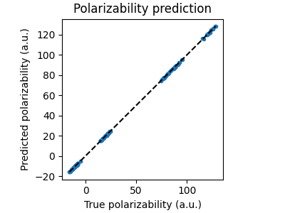
Let us plot the predicted polarizability tensor against the true polarizability tensor for the test set.

true_polarizability = np.concatenate(
    [
        cartesian_tensormap_test.block(k).values.flatten().numpy()
        for k in cartesian_tensormap_test.keys
    ]
)
predicted_polarizability = np.concatenate(
    [
        prediction_test["cookbook::polarizability"]
        .block(k)
        .values.flatten()
        .detach()
        .numpy()
        for k in prediction_test["cookbook::polarizability"].keys
    ]
)

fig, ax = plt.subplots(1, 1, figsize=(4, 3), constrained_layout=True)
ax.set_aspect("equal")
ax.plot(true_polarizability, predicted_polarizability, ".")
ax.plot(
    [true_polarizability.min(), true_polarizability.max()],
    [true_polarizability.min(), true_polarizability.max()],
    "--k",
)
ax.set_xlabel("True polarizability (a.u.)")
ax.set_ylabel("Predicted polarizability (a.u.)")
ax.set_title("Polarizability prediction")
plt.show()

Export the model as a metatomic model

Wrap the model in a metatensor.torch.atomistic.MetatensorAtomisticModel object.

outputs = {
    "cookbook::polarizability": ModelOutput(
        quantity="polarizability", unit="a.u.", per_atom=False
    )
}

options = ModelEvaluationOptions(
    length_unit="angstrom", outputs=outputs, selected_atoms=None
)

model_capabilities = ModelCapabilities(
    outputs=outputs,
    atomic_types=[1, 6, 7, 16],
    interaction_range=4.5,
    length_unit="angstrom",
    supported_devices=["cpu"],
    dtype="float64",
)

atomistic_model = MetatensorAtomisticModel(
    model.eval(), ModelMetadata(), model_capabilities
)

The model can be saved to disk using the metatensor.torch.atomistic.save_atomistic_model() function.

atomistic_model.save("polarizability_model.pt", collect_extensions="extensions")

Use the model as a metatensor calculator

The model can be used as a calculator with the metatensor.torch.atomistic.MetatensorCalculator class.

atomistic_model = load_atomistic_model(
    "polarizability_model.pt", extensions_directory="extensions"
)
mta_calculator = MetatensorCalculator(atomistic_model)

ase_frames = ase.io.read("data/qm7x_reduced_100.xyz", index=":")

ase.Atoms objects do not feature a get_polarizability() method that we could call to compute the polarizability with our model. The easiest way to compute the polarizability is then to directly use the MetatensorCalculator.run_model() method, which takes a list of ase.Atoms objects and a dictionary of metatensor.torch.atomistic.ModelOutput objects as input. The output is a dictionary of metatensor.torch.TensorMap objects.

computed_polarizabilities = []
for frame in ase_frames:
    computed_polarizabilities.append(
        mta_calculator.run_model(frame, outputs)["cookbook::polarizability"]
        .block(0)
        .values.squeeze()
        .numpy()
    )
computed_polarizabilities = np.stack(computed_polarizabilities)

This is essentially the same model as before, wrapped in a stand-alone format

train_mae = np.abs(
    (cartesian_polarizability - computed_polarizabilities)[train_idx]
).mean()
test_mae = np.abs(
    (cartesian_polarizability - computed_polarizabilities)[test_idx]
).mean()

print(
    f"""
Model train MAE: {train_mae} a.u.
Model test MAE:  {test_mae} a.u.
"""
)

Model train MAE: 0.05014023428939952 a.u.
Model test MAE:  0.22713940841134175 a.u.