Conservative fine-tuning for a PET model

Authors:

Michele Ceriotti @ceriottm, Sofiia Chorna @sofiia-chorna

This example demonstrates a “conservative fine-tuning” (or equivalently, “non-conservative pre-training”) strategy. This consists in training a model using (faster) direct, non-conservative force predictions, and then fine-tuning it with backpropagated forces to achieve an accurate conservative model.

As discussed in this paper, while conservative MLIPs are generally better suited for physically accurate simulations, hybrid models that support direct non-conservative force predictions can accelerate both training and inference. Training can be accelerated through a two-stage approach: first train a model to predict non-conservative forces directly (avoiding the cost of backpropagation) and then fine-tune its energy head to produce conservative forces. This two-step strategy is usually faster and produces a model that can exploit both types of force predictions. An example of how to use direct forces in molecular dynamics simulations safely (i.e. avoiding unphysical behavior due to lack of energy conservation) is provided in this example.

If you are looking for traditional fine-tuning of a pre-trained universal model, see for example this recipe. Note also that the models generated in this example are run for too short a time to produce a useful model (further revealing the advantages of this direct-force pre-training strategy). The data file contains also “long” training settings, which can be used (preferably on a GPU) to train a model up to a point that reveals the behavior of the method in more realistic conditions. It should also be noted that this technique is particularly useful to speed up the training of large models on large (potentially universal) datasets.

# sphinx_gallery_thumbnail_path = '../../examples/pet-finetuning/training_strategy_comparison.png'  # noqa

import subprocess
from time import time

import ase.io
import numpy as np

Prepare the training set

We begin by creating a train/validation/test split of the dataset.

dataset = ase.io.read("data/ethanol.xyz", index=":", format="extxyz")

np.random.seed(42)
indices = np.random.permutation(len(dataset))
n = len(dataset)
n_val = n_test = int(0.1 * n)
n_train = n - n_val - n_test

train = [dataset[i] for i in indices[:n_train]]
val = [dataset[i] for i in indices[n_train : n_train + n_val]]
test = [dataset[i] for i in indices[n_train + n_val :]]

ase.io.write("data/ethanol_train.xyz", train, format="extxyz")
ase.io.write("data/ethanol_val.xyz", val, format="extxyz")
ase.io.write("data/ethanol_test.xyz", test, format="extxyz")

Non-conservative force training

metatrain provides a convenient interface to train a PET model with non-conservative forces. You can see the metatrain documentation for general examples of how to use this tool. The key step to add non-conservative forces is to add a non_conservative_forces section to the targets specifications of the YAML file describing the training exercise

seed: 42

architecture:
  name: pet
  training:
    batch_size: 10 
    num_epochs: 20
    learning_rate: 1e-4

training_set:
  systems:
    read_from: data/ethanol_train.xyz
    length_unit: angstrom
  targets:
    energy:
      unit: eV
      forces: off
    non_conservative_forces:
      key: forces
      quantity: force
      unit: eV/A  
      type:
        cartesian:
          rank: 1
      per_atom: true

validation_set:
  systems: 
    read_from: data/ethanol_val.xyz
    length_unit: angstrom
  targets:
    energy:
      key: energy
      unit: eV
      forces: off
    non_conservative_forces:
      key: forces
      quantity: force  
      unit: eV/A  
      type:
        cartesian:
          rank: 1
      per_atom: true

test_set:
  systems: 
    read_from: data/ethanol_test.xyz
    length_unit: angstrom
  targets:
    energy:
      key: energy
      unit: eV
      forces: off
    non_conservative_forces:
      key: forces
      quantity: force  
      unit: eV/A  
      type:
        cartesian:
          rank: 1
      per_atom: true

Adding a non_conservative_forces target with these specifications automatically adds a vectorial output to the atomic heads of the model, but does not disable the energy head, which is still used to compute the energy, and could in principle be used to compute conservative forces. To profit from the speed up of direct force evaluation, we specify forces: off in the energy target, turning off the backpropagation of forces.

Training can be run from the command line using the mtt command:

mtt train nc_train_options.yaml -o nc_model.pt

or from Python:

time_nc = -time()
subprocess.run(
    ["mtt", "train", "nc_train_options.yaml", "-o", "nc_model.pt"], check=True
)
time_nc += time()
print(f"Training time (non-cons.): {time_nc:.2f} seconds")

Training time (non-cons.): 21.63 seconds

At evaluation time, we can compute both conservative and non-conservative forces. Note that the training run is too short to produce a decent model. If you have a GPU and a few more minutes, you can run one of the long_* option files, that provide a more realistic training setup. You can evaluate from the command line

mtt eval nc_model.pt nc_model_eval.yaml

Or from Python:

subprocess.run("mtt eval nc_model.pt nc_model_eval.yaml".split(), check=True)

CompletedProcess(args=['mtt', 'eval', 'nc_model.pt', 'nc_model_eval.yaml'], returncode=0)

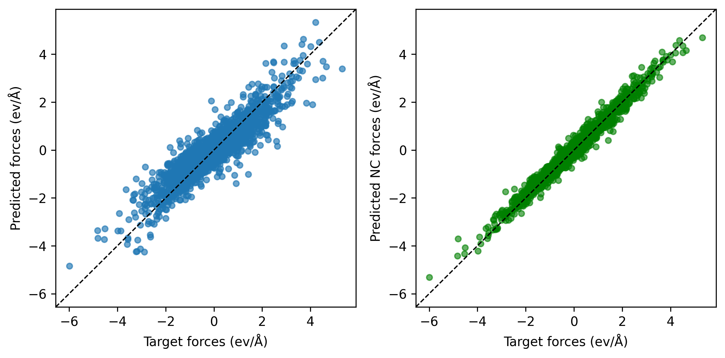
The result of a non-conservative force learning run (600 epochs) is presented in the parity plot below. The plot shows that the model’s conservative force predictions (that are not trained, on the left) have larger errors than those obtained from the trained direct predictions (right). The non-conservative forces align closely with the targets but lack the physical constraint of being the derivatives of a potential energy, often leading to unphysical behavior when used in simulations.

Fine-tuning on conservative forces

Even though the error on energy derivatives is pretty large, the model has learned a reasonable representation of the energy of the systems, and we can use it as a starting point to fine-tune the model to improve the accuracy on conservative forces. We enable forces: on to compute them via backward propagation of gradients. We also keep training the non-conservative forces (with a small loss weight) so that we can still use the model for fast direct force inference, with minimal overhead against forward energy evaluation. Expectedly, the training will be slower.

training_set:
  systems:
    read_from: data/ethanol_train.xyz
    length_unit: angstrom
  targets:
    energy:
      unit: eV
      forces: on
    non_conservative_forces:
      key: forces
      type:
        cartesian:
          rank: 1
      per_atom: true

Run training, restarting from the previous checkpoint:

mtt train c_ft_options.yaml -o c_ft_model.pt --restart=nc_model.ckpt

Or in Python:

time_c_ft = -time()
subprocess.run(
    "mtt train c_ft_options.yaml -o c_ft_model.pt --restart=nc_model.ckpt".split(" "),
    check=True,
)
time_c_ft += time()
print(f"Training time (conservative fine-tuning): {time_c_ft:.2f} seconds")

Training time (conservative fine-tuning): 36.04 seconds

Let’s evaluate the forces again.

mtt eval nc_model.pt nc_model_eval.yaml

Or from Python:

subprocess.run("mtt eval nc_model.pt nc_model_eval.yaml".split(), check=True)

CompletedProcess(args=['mtt', 'eval', 'nc_model.pt', 'nc_model_eval.yaml'], returncode=0)

Converged results

Note

To reproduce the results shown below, run extended training simulations using the provided YAML configuration files. These runs are longer, and too slow to be executed on a CPU in the automated testing framework of the cookbook, so we provide static images to comment on the outcomes.

We extend the training time with more epochs to obtain improved predictive performance. Below are the full YAML parameter sets used for the long non-conservative and conservative runs:

Non-conservative training (NC) YAML

seed: 42

architecture:
  name: pet
  training:
    batch_size: 8
    num_epochs: 700
    learning_rate: 3e-4

training_set:
  systems:
    read_from: data/ethanol_train.xyz
    length_unit: angstrom
  targets:
    energy:
      unit: eV
      forces: off
    non_conservative_forces:
      key: forces
      quantity: force
      unit: eV/A  
      type:
        cartesian:
          rank: 1
      per_atom: true

validation_set:
  systems: 
    read_from: data/ethanol_val.xyz
    length_unit: angstrom
  targets:
    energy:
      key: energy
      unit: eV
      forces: off
    non_conservative_forces:
      key: forces
      quantity: force  
      unit: eV/A  
      type:
        cartesian:
          rank: 1
      per_atom: true

test_set:
  systems: 
    read_from: data/ethanol_test.xyz
    length_unit: angstrom
  targets:
    energy:
      key: energy
      unit: eV
      forces: off
    non_conservative_forces:
      key: forces
      quantity: force  
      unit: eV/A  
      type:
        cartesian:
          rank: 1
      per_atom: true

Conservative fine-tuning (C) YAML

seed: 42

architecture:
  name: pet
  training:
    num_epochs: 3000
    learning_rate: 1e-5
    batch_size: 10

training_set:
  systems:
    read_from: data/ethanol_train.xyz
    length_unit: angstrom
  targets:
    energy:
      key: energy
      unit: eV
      forces: on
    non_conservative_forces:
      key: forces
      quantity: force  
      unit: eV/A  
      type:
        cartesian:
          rank: 1
      per_atom: true

validation_set:
  systems: 
    read_from: data/ethanol_val.xyz
    length_unit: angstrom
  targets:
    energy:
      key: energy
      unit: eV
      forces: on
    non_conservative_forces:
      key: forces
      quantity: force  
      unit: eV/A  
      type:
        cartesian:
          rank: 1
      per_atom: true

test_set:
  systems: 
    read_from: data/ethanol_test.xyz
    length_unit: angstrom
  targets:
    energy:
      key: energy
      unit: eV
      forces: on
    non_conservative_forces:
      key: forces
      quantity: force  
      unit: eV/A  
      type:
        cartesian:
          rank: 1
      per_atom: true

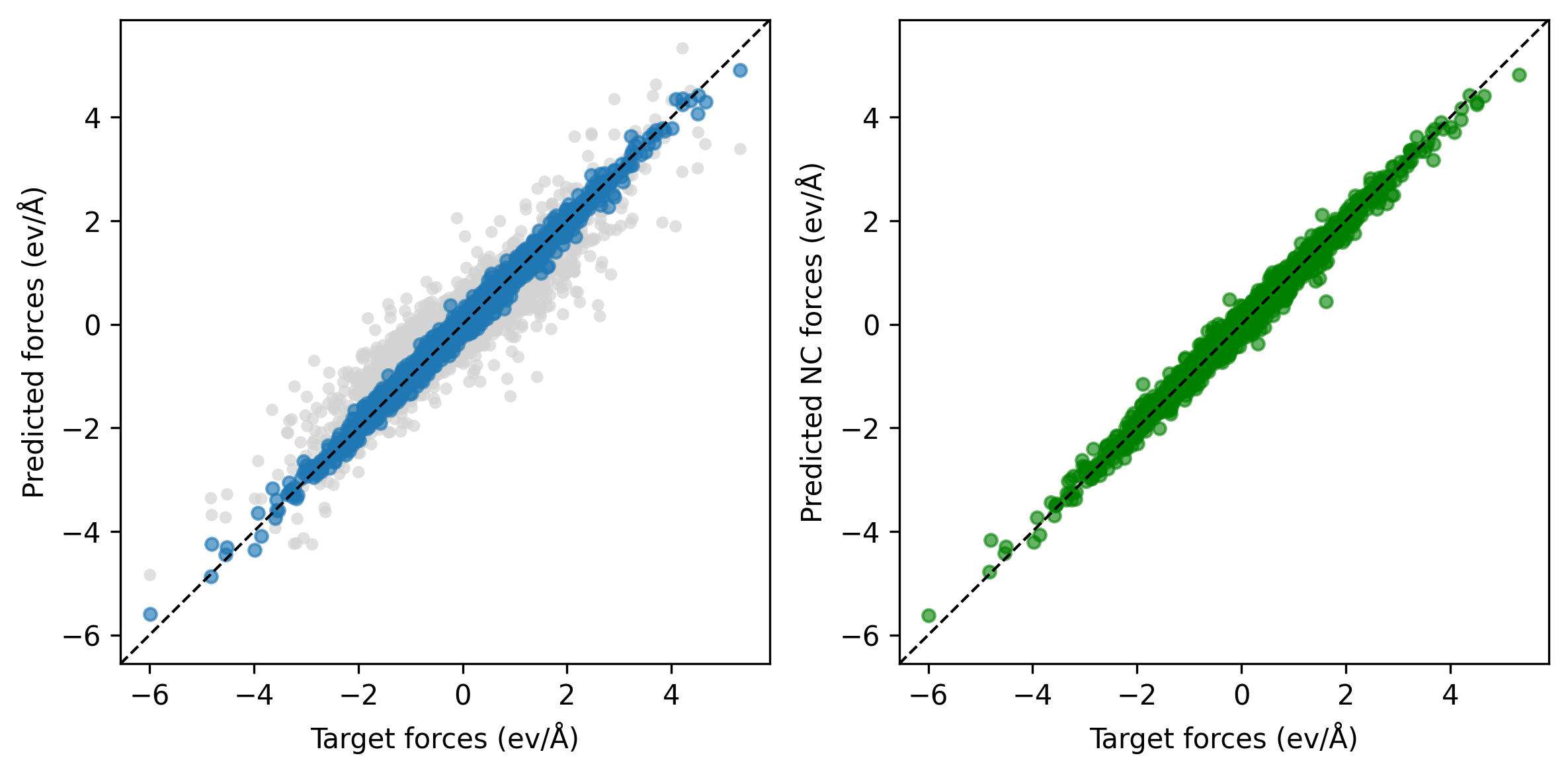
After conservative fine-tuning for 2400 epochs, the updated parity plots show improved force predictions (left) with conservative forces. The grayscale points in the background correspond to the predicted forces from the non-conservative step.

The figure below compares the validation force MAE as a function of GPU hours for direct training of the conservative PET model (“C-only”) and a two-step approach: initial training of a non-conservative model followed by conservative training continuation. For the given GPU hours frame, the two-step approach yields lower validation error (or achieve the same accuracy in a shorter time).

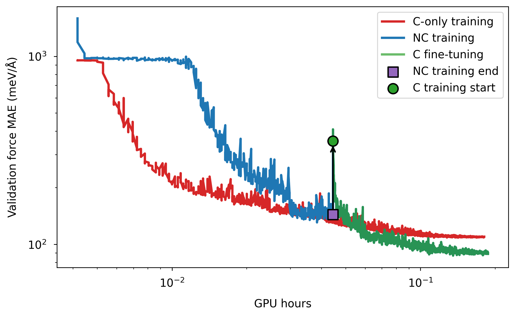
Training on a larger dataset and performing some hyperparameter optimization could further improve performance.