Water orientation in a pulsed electric field

Authors:

Philip Loche @PicoCentauri

Energy dissipation in water is very fast and more efficient than in many other liquids. This behavior is commonly attributed to the intermolecular interactions associated with hydrogen bonding. This effect has been studied intensively by experiments, ab initio, and classical simulations in the work by Elgabarty et al.. Here, we will re run some of the classical force field molecular dynamics (MD) simulations of the paper using the GROMACS package to compute the timeseries of the dipole moments as well as the energy.

Note

We will only run a single simulation/pulse. To get enough statistics for clear results as in the paper, one has to run around ~10,000 pulses.

We start by loading the required packages. The base tool for loading trajectories will be MDAnalysis, and for computing the dipole moment, we will use MAICoS.

import subprocess

import maicos
import matplotlib.pyplot as plt
import MDAnalysis as mda
import numpy as np

A simulated laser pulse

We will simulate a periodic water box at constant particle number, volume, and energy (NVE) in an alternating electric field according to

\[E(t) = E_0 \exp \left[ -\frac{(t-t_0)^2}{2 \sigma^2} \right] \cos\left[\omega (t-t_0)\right]\]

where \(E_0\) is the field strength, \(\omega\) is the angular frequency, \(t_0\) is the time at the peak of the field strength, and \(\sigma\) is the width of the pulse. We define the electric pulse with this function.

def Efield(t, E0, omega, t0, sigma):
    """An alternating and pulsed electric field."""
    E = E0 * np.cos(omega * (t - t0))
    if sigma == 0:
        return E
    else:
        return E * np.exp(-((t - t0) ** 2) / (2 * sigma**2))

We now plot the electric field over time using the same parameters as later in our simulations.

time = np.linspace(0, 10, 101)
electric_field = Efield(time, E0=0.5, omega=1.0, t0=5.0, sigma=0.5)

plt.axhline(0, color="k", linestyle="--")
plt.plot(time, electric_field)
plt.xlabel("Time (ps)")
plt.ylabel("Electric Field (V/nm)")
plt.show()

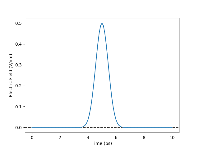
As you can see, the pulse lasts for roughly 2 ps, which is consistent with the experimental findings.

Simulate a water box

The simulation system is a cubic box with a 5.5 nm edge length containing 5360 water molecules. We first create the topology using the pdb2gmx tool with rigid SPC/E molecules.

subprocess.check_call(
    ["gmx", "pdb2gmx", "-f", "data/conf.gro.gz", "-ff", "amber99", "-water", "spce"]
)

0

We use the AMBER99 force field even though we don’t use any parameters besides the definitions of SPC/E. We will run a simulation based on MD parameter (mdp) saved in the grompp.mdp file. The simulation will be run for 10 ps with a timestep of 2 fs. For a detailed explanation of the parameters, refer to the GROMACS documentation. The electric field pointing in the \(x\) direction is defined at the very end with the electric-field-x directive.

Before running the simulation, we use the GROMACS preprocessor (grompp) to create the necessary tpr input file.

subprocess.check_call(["gmx", "grompp", "-f", "data/grompp.mdp"])

0

And run the simulation, which should take about 30 seconds to complete.

subprocess.check_call(["gmx", "mdrun"])

0

Water orientation

Now that we have the trajectory, we can load the positions and analyze the data.

u = mda.Universe("topol.tpr", "traj_comp.xtc")

n_frames = u.trajectory.n_frames
n_residues = u.atoms.residues.n_residues

We define a helper function that provides a vector pointing in the x-direction for every molecule in the system. For this simple example, the creation could be done manually, but using a function makes it easily generalizable. Since our field points in the \(x\) direction, we set pdim to 0.

def get_unit_vectors(atomgroup: mda.AtomGroup, grouping: str):
    return maicos.lib.util.unit_vectors_planar(
        atomgroup=atomgroup, grouping=grouping, pdim=0
    )

We now define the arrays to store the data and run the analysis over the whole trajectory to compute the self and collective contributions of the dipole orientation.

time = np.empty(n_frames)
cos_theta_i = np.empty(n_frames)
cos_theta_ii = np.empty(n_frames)
cos_theta_ij = np.empty(n_frames)

for i_ts, ts in enumerate(u.trajectory):
    u.atoms.unwrap()

    cos_theta = maicos.lib.weights.diporder_weights(
        u.atoms,
        grouping="molecules",
        order_parameter="cos_theta",
        get_unit_vectors=get_unit_vectors,
    )
    matrix = np.outer(cos_theta, cos_theta)

    trace = matrix.trace()

    time[i_ts] = ts.time
    cos_theta_i[i_ts] = cos_theta.mean()
    cos_theta_ii[i_ts] = trace / n_residues
    cos_theta_ij[i_ts] = matrix.sum() - trace
    cos_theta_ij[i_ts] /= n_residues**2 - n_residues

We have all data and can plot the results in a shared figure

fig, ax = plt.subplots(3)
ax[0].plot(time, cos_theta_i, label="cos_theta_i")
ax[0].set_ylabel(r"$\langle \cos(\theta)_i \rangle$")
ax[1].plot(time, cos_theta_ii, label="cos_theta_ii")
ax[1].set_ylabel(r"$\langle \cos(\theta)_{ii} \rangle$")
ax[2].plot(time, cos_theta_ij, label="cos_theta_ij")
ax[2].set_ylabel(r"$\langle \cos(\theta)_{ij} \rangle$")

for a in ax:
    axE = a.twinx()
    axE.plot(time, electric_field, c="red", ls="dashed")
    axE.set_ylabel("E (V/nm)", color="red")
    axE.tick_params("y", colors="r", which="both")

ax[-1].set_xlabel("Time (ps)")
fig.align_labels()

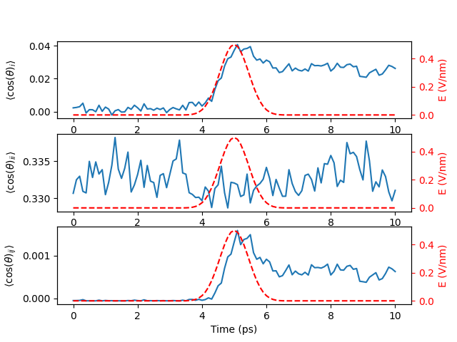
We find that the reorientation of water molecules is influenced by the applied electric field. Next, we will check the energy dissipation.

Energy over time

MDAnalysis offers the EDRReader class to read energy data from GROMACS energy files and attach it to a trajectory.

aux = mda.auxiliary.EDR.EDRReader("ener.edr")

/home/runner/work/atomistic-cookbook/atomistic-cookbook/.nox/water-pulsed/lib/python3.12/site-packages/MDAnalysis/auxiliary/EDR.py:350: UserWarning: Could not find unit type for the following units: ['K', 'bar', 'bar nm']
  warnings.warn(

To add this auxiliary data, we have to create a dictionary. This will be used to store the data and access it later, while the values are the names of the properties in the edr file. aux.terms shows a list of all properties.

u.trajectory.add_auxiliary(
    {"epot": "Potential", "etot": "Total Energy", "ekin": "Kinetic En."}, aux
)

etot = np.zeros(len(u.trajectory))
ekin = np.zeros(len(u.trajectory))
epot = np.zeros(len(u.trajectory))

for i_ts, ts in enumerate(u.trajectory):
    etot[i_ts] = ts.aux["etot"]
    ekin[i_ts] = ts.aux["ekin"]
    epot[i_ts] = ts.aux["epot"]

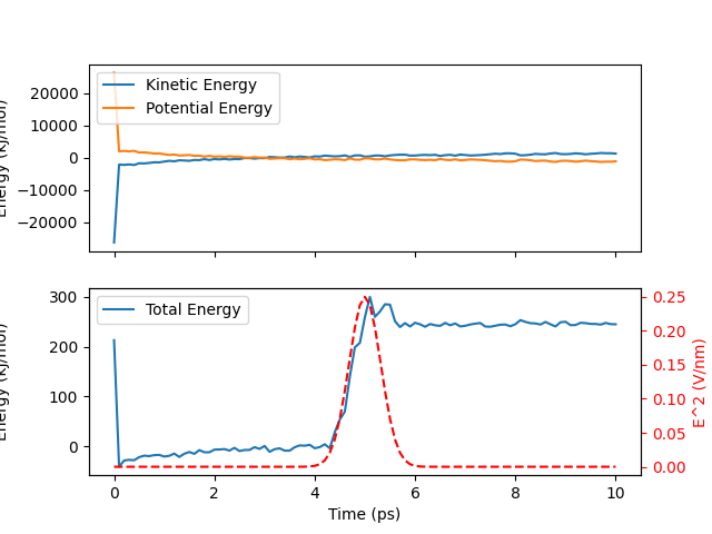
We now plot the data and observe energy transfer in this NVE simulation due to the applied pulse. As mentioned earlier, resolving the noisy data fully requires at least two to three orders of magnitude more simulations.

fig, ax = plt.subplots(2, sharex=True)
ax[0].plot(time, ekin - ekin.mean(), label="Kinetic Energy")
ax[0].plot(time, epot - epot.mean(), label="Potential Energy")
ax[0].legend(loc="upper left")
ax[0].set_ylabel("Energy (kJ/mol)")

ax[1].plot(time, etot - etot[:10].mean(), label="Total Energy")
ax[1].set_ylabel("Energy (kJ/mol)")
ax[1].legend(loc="upper left")

axE = ax[1].twinx()
axE.plot(time, electric_field**2, c="red", ls="dashed")
axE.set_ylabel("E^2 (V/nm)", color="red")
axE.tick_params("y", colors="r", which="both")

ax[-1].set_xlabel("Time (ps)")

fig.align_labels()