Note
Go to the end to download the full example code.
Ring Polymer Instanton Rate Theory: Tunneling Rates
- Authors:
Yair Litman @litman90
# sphinx_gallery_thumbnail_number = 2
This notebook introduces the calculation of tunneling rates using ring-polymer instanton rate theory. A comprehensive presentation of the instanton formalism can be found in the review article by J. Richardson, Int. Rev. Phys. Chem., 37, 171, 2018, while the implementation within i-PI is described in V. Kapil et al., Comp. Phys. Commun., 236, 214, 2020. Additional practical details are available in Yair Litman’s doctoral thesis.
import glob
import re
import shutil
import subprocess
import time
from pathlib import Path

import chemiscope
import ipi
import matplotlib.pyplot as plt
import numpy as np
from scipy import constants
from ipi.utils.tools import interpolate_instanton
Instanton calculations using i-PI
In these exercises, i-PI will be used not for molecular dynamics simulations, but to optimize stationary points on the ring-polymer potential-energy surface. From these stationary points, the ring-polymer instanton can be obtained and employed to evaluate thermal reaction rates that include tunneling contributions.
As a working example, we consider the gas-phase bimolecular reaction H + CH4 –>CH3 + H2. The calculations are performed using the CBE potential-energy surface reported in J. C. Corchado et al., J. Chem. Phys., 130, 184314, 2009.
If you are new to path-integral simulations or to the use of i-PI, which is the software which will be used to perform simulations, you can see this introductory recipe.
ipi_path = Path(ipi.__file__).resolve().parent
Installing the Python driver
i-PI provides a FORTRAN driver that includes the CBE potential-energy surface. However, the driver must be compiled from source. We use a utility function to compile it.
Note that this requires a working build environment with gfortran and make available.
ipi.install_driver()
Calculation Workflow
The calculation of tunneling rates using ring-polymer instanton theory is a multi-step procedure that requires the optimization of several stationary points on the system’s potential-energy surface. The workflow is not fully automated and therefore involves multiple independent runs of i-PI.
A typical workflow is summarized below:
1. Locate the minima on the physical potential-energy surface to identify the reactant and product states. Compute their Hessians, normal-mode frequencies, and eigenvectors.
2. Find the first-order saddle point corresponding to the transition state and evaluate its Hessian.
3. Obtain an “unconverged” instanton by locating the first-order saddle point of the ring-polymer Hamiltonian using N replicas. The chosen N should be large enough that the instanton provides a reasonable initial guess for a more converged calculation with a larger number of replicas, but small enough to keep the computational cost moderate. This step also provides an approximate Hessian for each replica.
4. Use ring-polymer interpolation to construct an instanton with a larger number of replicas. As a rule of thumb, the number of replicas can be doubled.
5. Re-optimize the instanton by locating the corresponding first-order saddle point.
6. Repeat steps 4 and 5 until the instanton is converged with respect to the number of replicas.
7. Recompute the Hessian for each replica accurately and evaluate the reaction rate.
If rates are required at multiple temperatures, it is recommended to start with temperatures close to the crossover temperature and then cool sequentially, using the optimized instanton from the previous temperature as the initial guess for the next calculation.
Step 1 - Optimizing and Analyzing the Reactant
We begin by performing a geometry optimization of the reactant.
The relevant sections of the input file that control the geometry optimization are highlighted below.
Open and inspect the XML input file:
with open("data/input_vibrations_reactant.xml", "r") as file:
    lines = file.readlines()

for line in lines[18:23]:
    print(line, end="")
<vibrations mode="fd">
    <pos_shift> 0.01  </pos_shift>  <!-- Displacment length -->
    <prefix> vib </prefix>
    <asr> none </asr>               <!-- Apply acoustic sume rule: none, crystal (translation) or poly(rotation and translation) -->
 </vibrations>
We can launch i-pi and the driver from a Python script as follows
ipi_process = None
ipi_process = subprocess.Popen(["i-pi", "data/input_geop_reactant.xml"])
time.sleep(5)  # wait for i-PI to start

FF_process = subprocess.Popen(["i-pi-driver", "-u", "-m", "ch4hcbe"])
FF_process.wait()
ipi_process.wait()
0
The simulation converges in 31 steps, and the optimized geometry can
be found in the last frame of min.xc.xyz. After completing this
exercise, you may return to this point and attempt to reduce the number
of optimization steps, for example by replacing sd with one of the
alternative optimizers.
Since this is a bimolecular reaction, the H atom and CH\(_4\) molecule must remain well separated. For this reason, a very large simulation box has been used.
Extract the final frame of the geometry optimization trajectory and use it to compute the harmonic vibrational frequencies.
with open("min_reactant.xyz", "w") as outfile:
    subprocess.run(
        ["tail", "-n", "8", "geop_reactant.xc.xyz"], stdout=outfile, check=True
    )


time.sleep(5)  # wait for i-PI to start
#    We will now compute the hessian of this  minimum eneryg geometry

ipi_process = None
ipi_process = subprocess.Popen(["i-pi", "data/input_vibrations_reactant.xml"])
time.sleep(5)  # wait for i-PI to start

FF_process = subprocess.Popen(["i-pi-driver", "-u", "-m", "ch4hcbe"])
FF_process.wait()
ipi_process.wait()
0
The hessian is saved in vib_reactant.hess and
its eigenvalues in vib_reactant.eigval.
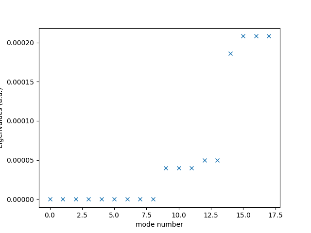
Check that it has the required number (9) of almost zero eigenvalues. Why?
eigvals = np.genfromtxt("vib_reactant.vib.eigval")
plt.plot(eigvals, "x")
plt.xlabel("mode number")
plt.ylabel("Eigenvalues (a.u.)")
plt.show()

shutil.copy("RESTART", "RESTART_reactant")
'RESTART_reactant'
Step 2 - Optimizing and Analyzing the Transition State
We now optimize the transition-state (TS) geometry. The procedure is analogous to that used for the reactant, but we employ a different input file configured specifically for a transition-state optimization.
The relevant sections of the input file that define the transition-state optimization are highlighted below:
with open("data/input_geop_TS.xml", "r") as file:
    lines = file.readlines()

for line in lines[18:31]:
    print(line, end="")
<instanton mode='rate'>                      <!-- This option implies that we are looking a transition state -->
    <tolerances>
        <energy> 5e-6 </energy>
        <force> 5e-6 </force>
        <position> 1e-3 </position>
    </tolerances>
    <alt_out>-1</alt_out>                    <!-- Print frequency of alternative output. -->
    <hessian_update>powell</hessian_update>  <!-- Specify the way we update our hessian. Options: powell or recompute. -->
    <hessian_asr>poly</hessian_asr>          <!-- Type of acoustic sum rule applied -->
    <hessian_init>true</hessian_init>        <!-- Boolean that specifies if the initial hessian is going to be computed from scratch or not -->
    <hessian_final>true</hessian_final>      <!-- Boolean that specifies if after the optimization is converged a hessian should be computed or not -->
    <biggest_step>0.3</biggest_step>
</instanton>
Note that Here i-PI treats the TS search as a one-bead instanton optimization.
We now launch i-PI together with the driver using commands analogous to those used in the previous step:
ipi_process = None
ipi_process = subprocess.Popen(["i-pi", "data/input_geop_TS.xml"])
time.sleep(5)  # wait for i-PI to start

FF_process = subprocess.Popen(["i-pi-driver", "-u", "-m", "ch4hcbe"])
FF_process.wait()
ipi_process.wait()
shutil.copy("RESTART", "RESTART_ts")
'RESTART_ts'
The simulation typically converges in 11–12 steps and writes the
optimized geometry to ts.instanton_FINAL_xx.xyz and the corresponding
Hessian to ts.instanton_FINAL.hess_xx.
ts_energy_ev = np.loadtxt("ts.out")[1, -1]
Step 3 - First instanton optimization
We now continue with the optimization of the ring-polymer instanton. This is a first-order saddle point of the ring-polymer Hamiltonian, and therefore the optimization procedure is analogous to that used for the transition state. To generate the initial guess for the instanton optimization, we use the transition state geometry and hessian obtained in the previous step. The
# Retrieve the Hessian and geometry files from the converged
# transition-state calculation and rename them as required.

final_step = max(
    int(re.search(r"hess_(\d+)$", f).group(1))
    for f in glob.glob("ts.instanton_FINAL.hess_*")
)

ts_hess_file = f"ts.instanton_FINAL.hess_{final_step}"
ts_xyz_file = f"ts.instanton_FINAL_{final_step}.xyz"


shutil.copy(ts_xyz_file, "init_inst_geop.xyz")
shutil.copy(ts_hess_file, "init_inst_geop.hess")
'init_inst_geop.hess'
We run i-PI in the usual way, but here we launch four driver instances simultaneously using:
ipi_process = None
ipi_process = subprocess.Popen(["i-pi", "data/input_geop_RPI_40.xml"])
time.sleep(5)  # wait for i-PI to start

FF_process = [
    subprocess.Popen(["i-pi-driver", "-u", "-m", "ch4hcbe"]) for i in range(4)
]

ipi_process.wait()

shutil.copy("RESTART", "RESTART_RPI_40")
'RESTART_RPI_40'
The program first generates an initial instanton guess by placing
replicas around the transition state along the direction of the
imaginary mode. It then performs a saddle-point optimization.
The optimized instanton geometry is written to
ts.instanton_FINAL_X.xyz and can be visualized using vmd.
Finally, the Hessians for each bead are computed and saved in
ts.instanton_FINAL.hess_X with dimensions (3n, 3Nn), where n
is the number of atoms and N the number of beads.
Let’s visualize the instanton geometry. We first retrieve the filename of the optimized geometry and then use chemiscope to visualize it.
final_step = max(
    int(re.search(r"hess_(\d+)$", f).group(1))
    for f in glob.glob("inst.instanton_FINAL.hess_*")
)

inst_xyz_file_40 = f"inst.instanton_FINAL_{final_step}.xyz"


# NB: there is a parsing bug in i-PI 3.1 that causes the units to be
# converted incorrectly. The following code is a workaround to convert
# the units back to angstroms.
pi_frames = ipi.read_trajectory(
    inst_xyz_file_40, dimension="length", cell_units="atomic_unit", units="angstrom"
)
for f in pi_frames:
    f.positions *= 0.529177  # convert from bohr to angstrom

chemiscope.show(
    structures=pi_frames,
    settings=chemiscope.quick_settings(
        trajectory=True,
    ),
    mode="structure",
)

!W! cell is not a known trajectory type. Will apply no units conversion
!W! cell is not a known trajectory type. Will apply no units conversion
!W! cell is not a known trajectory type. Will apply no units conversion
!W! cell is not a known trajectory type. Will apply no units conversion
!W! cell is not a known trajectory type. Will apply no units conversion
!W! cell is not a known trajectory type. Will apply no units conversion
!W! cell is not a known trajectory type. Will apply no units conversion
!W! cell is not a known trajectory type. Will apply no units conversion
!W! cell is not a known trajectory type. Will apply no units conversion
!W! cell is not a known trajectory type. Will apply no units conversion
!W! cell is not a known trajectory type. Will apply no units conversion
!W! cell is not a known trajectory type. Will apply no units conversion
!W! cell is not a known trajectory type. Will apply no units conversion
!W! cell is not a known trajectory type. Will apply no units conversion
!W! cell is not a known trajectory type. Will apply no units conversion
!W! cell is not a known trajectory type. Will apply no units conversion
!W! cell is not a known trajectory type. Will apply no units conversion
!W! cell is not a known trajectory type. Will apply no units conversion
!W! cell is not a known trajectory type. Will apply no units conversion
!W! cell is not a known trajectory type. Will apply no units conversion
!W! cell is not a known trajectory type. Will apply no units conversion
!W! cell is not a known trajectory type. Will apply no units conversion
!W! cell is not a known trajectory type. Will apply no units conversion
!W! cell is not a known trajectory type. Will apply no units conversion
!W! cell is not a known trajectory type. Will apply no units conversion
!W! cell is not a known trajectory type. Will apply no units conversion
!W! cell is not a known trajectory type. Will apply no units conversion
!W! cell is not a known trajectory type. Will apply no units conversion
!W! cell is not a known trajectory type. Will apply no units conversion
!W! cell is not a known trajectory type. Will apply no units conversion
!W! cell is not a known trajectory type. Will apply no units conversion
!W! cell is not a known trajectory type. Will apply no units conversion
!W! cell is not a known trajectory type. Will apply no units conversion
!W! cell is not a known trajectory type. Will apply no units conversion
!W! cell is not a known trajectory type. Will apply no units conversion
!W! cell is not a known trajectory type. Will apply no units conversion
!W! cell is not a known trajectory type. Will apply no units conversion
!W! cell is not a known trajectory type. Will apply no units conversion
!W! cell is not a known trajectory type. Will apply no units conversion
!W! cell is not a known trajectory type. Will apply no units conversion
Step 4 - Second and subsequent instanton optimizations
The instanton obtained in the previous step might not be fully converged with respect to the number of beads. To obtain a more converged instanton, we can interpolate the geometry and the Hessian to a larger number of beads and then re-optimize. This procedure can be repeated until the instanton is converged
The procedure would be as follows: 1. Let’s retrieve the filenames of the Hessian and geometry corresponding to the converged instanton.
inst_hess_file_40 = f"inst.instanton_FINAL.hess_{final_step}"

#
2. The utility function interpolate_instanton can now be used to
interpolate both the geometry and the Hessian to a larger number
of beads. For example, to increase the number of beads from 40 to 80,
you could run the script inside ${ipi-path}/uitls/tools/:
python onstanton_interpolation.py -m -xyz init0 -hess hess0 -n 80
Here, however, we import and use the corresponding function directly within Python.
interpolate_instanton(
    input_geo=inst_xyz_file_40,
    input_hess=inst_hess_file_40,
    nbeadsNew=80,
    manual="True",
)
We have a half ring polymer made of 40 beads and 6 atoms.
We will expand the ring polymer to get a half polymer of 80 beads.
The new Instanton geometry (half polymer) was generated
Check new_instanton.xyz

Don't forget to change the number of beads to the new value (80) in your input file
when starting your new simulation with an increased number of beads.

The new hessian is 18 x 1440.
Creating matrix...
The new physical Hessian (half polymer) was generated
Check new_hessian.dat

Remeber to adapt/add the following line in your input file:

 <hessian mode='file' shape='(18, 1440)' >hessian.dat</hessian>
3. The previous function generates the interpolated geometry and hessian. we now rename the new files as required by new input.xml
shutil.copy("new_instanton.xyz", "init_inst_80beads.xyz")
shutil.copy("new_hessian.dat", "init_inst_80beads.hess")
'init_inst_80beads.hess'
We now run the instanton optimization with 80 beads.
ipi_process = None
ipi_process = subprocess.Popen(["i-pi", "data/input_geop_RPI_80.xml"])
time.sleep(5)  # wait for i-PI to start

FF_process = [
    subprocess.Popen(["i-pi-driver", "-u", "-m", "ch4hcbe"]) for i in range(4)
]
# FF_process.wait()
ipi_process.wait()
time.sleep(5)

shutil.copy("RESTART", "RESTART_RPI_80")
'RESTART_RPI_80'
Step 5 - Postprocessing for the rate calculation
In the remainder of this step, we use the Instanton postprocessing
tool to compute the partition functions and the tunneling factor.
This Python script evaluates the different contributions to the rate,
including the partition functions and the instanton action, from the
outputs generated in the previous steps. It is located in the
utils/tools/instanton_postproc.py directory of the i-PI installation.
Note that we optimize only half of the ring polymer, since the forward
and backward imaginary-time paths between reactant and product are
identical. As a result, optimizing a ring polymer with 80 replicas
corresponds to a full instanton containing 160 replicas.
(This convention is currently somewhat confusing and may change in future versions.)
When using the Instanton postprocessing tool, always consult the
help option (-h) to verify the expected inputs.
Compute the CH\(_4\) partition function.
We compute the partition function at 300 K using 160 beads. Although within the harmonic approximation the exact value could be obtained analytically, it is preferable to use the finite-bead representation in order to remain consistent with the instanton calculation and benefit from error cancellation.
This can be done using the standalone script located in ${ipi-path}/tools/py/
python instanton_postproc.py RESTART_reactant -c reactant -t 300 -n 160 -f 5
which computes the ring polymer parition function for CH\(_4\) with N = 160. Look at the output and make a note of the translational, rotational and vibrational partition functions. You may also want to put > data.out after the command to save the text directly to a file.
RESTART_filename = (
    "RESTART_reactant"  # this is the restart file from the reactant calculation.
)
case = "reactant"
temperature = 300
nbeadsR = 160  # number of beads in the reactant calculation.
# This should be consistent with the number of beads used in the instanton calculation.

asr = "poly"
# we are treating the system as a polyatomic molecule,
# so we need to use the corresponding acoustic sum rule (ASR)

index_to_filter = 5  # we need to filter the H free atom.
V00 = 0.0  # This can be used to shift the energy.
# Since we are interested in the partition function of the reactant,
# we can set it to zero.
# However, when analyzing the transition state and the instanton in the manual mode,
# it is important to use the corresponding value of V00
# in order to ensure that the partition functions are computed consistently.

cmd = [
    "python",
    f"{ipi_path}/utils/tools/instanton_postproc.py",
    RESTART_filename,
    "-c",
    case,
    "-t",
    str(temperature),
    "-n",
    str(nbeadsR),
    "-asr",
    asr,
    "-f",
    str(index_to_filter),
    "--energy_shift",
    str(V00),
]

with open("data_reactant.out", "w") as outfile:
    subprocess.run(cmd, stdout=outfile, check=True)
Let’s read the output
with open("data_reactant.out", "r") as file:
    lines = file.readlines()

for line in lines[0:21]:
    print(line, end="")
We are ready to start. Reading RESTART_reactant ... (This can take a while)

Temperature: 300.0 K
NBEADS: 1
atoms:  5
ASR:    poly
1/(betaP*hbar) =  0.00095
Diagonalization ...


Lowest 10 frequencies (cm^-1)
[1383.00 1383.02 1383.13 1550.10 1550.18 2991.87 3164.13 3164.29 3164.37]
We saved the frequencies in freq.dat

We are done. Reactants. Nbeads 160
Qtras(bohr^-3) | Qrot     | logQvib_rp
         9.298 |  438.764 | -47.337

A file with the eigenvalues in atomic units was generated
2. Compute the TS partition function. This can be done using the standalone script located in ${ipi-path}/tools/py/ as follows:
python instanton_postproc.py RESTART_ts -c TS -t 300 -n 160
which computes the ring polymer parition function for the TS with \(N = 160\).
RESTART_filename = (
    "RESTART_ts"  # this is the restart file from the reactant calculation.
)
case = "TS"
temperature = 300
nbeadsR = 160

cmd = [
    "python",
    f"{ipi_path}/utils/tools/instanton_postproc.py",
    RESTART_filename,
    "-c",
    case,
    "-t",
    str(temperature),
    "-n",
    str(nbeadsR),
    "-asr",
    asr,
]

with open("data_ts.out", "w") as outfile:
    subprocess.run(cmd, stdout=outfile, check=True)
Let’s read the output
with open("data_ts.out", "r") as file:
    lines = file.readlines()

for line in lines:
    print(line, end="")
We are ready to start. Reading RESTART_ts ... (This can take a while)
324

Temperature: 300.0 K
NBEADS: 1
atoms:  6
ASR:    poly
1/(betaP*hbar) =  0.00095
Diagonalization ...


Lowest 10 frequencies (cm^-1)
[-1486.89 541.88 541.89 1084.08 1084.13 1182.15 1441.55 1441.56 1831.15 3034.03]
We saved the frequencies in freq.dat

We are done. TS
Partition functions at 300.0 K

Qtras: 10.187982156996487
Qrot: 1206.1516001364798
logQvib: -44.278348028965425
Potential energy at TS:  0.6505827861985822 eV, V/kBT 25.165639493793847
Look for the value of the imaginary frequency and use this to compute the crossover temperature defined by
Be careful of units! You should find that it is about 340 K. In the cell below we define a quick function that helps you with the necessary unit conversions.
# Physical Constants ###########
cm2hartree = 1.0 / (
    constants.physical_constants["hartree-inverse meter relationship"][0] / 100
)
Boltzmannau = (
    constants.physical_constants["Boltzmann constant in eV/K"][0]
    * constants.physical_constants["electron volt-hartree relationship"][0]
)


# Temperature <-> beta conversion ############
def beta2K(B):
    return 1.0 / B / Boltzmannau


def omb2Trecr(omega):
    return beta2K(2.0 * np.pi / (omega * cm2hartree))


omega = 1486.88  # given in reciprocal cm
print(
    (
        "The barrier frequency is %.2f cm^-1.\n"
        "The first recrossing temperature is ~ %.2f K."
    )
    % (omega, omb2Trecr(omega))
)
The barrier frequency is 1486.88 cm^-1.
The first recrossing temperature is ~ 340.48 K.
3. To compute the instanton partition function, \(B_N\) and action, we continue by calling the instanton postprocessing script located ${ipi-path}/utils/tools
python instanton_postproc.py RESTART_RPI_80 -c instanton -t 300
We don’t need to specify the number of beads here, since the script can read this from the restart file. The script will read the optimized instanton geometry and the corresponding Hessians, and use these to compute the partition functions and the action. Make a note of the different contributions to the rate that are printed in the output.
RESTART_filename = (
    "RESTART_RPI_80"  # this is the restart file from the reactant calculation.
)
case = "instanton"
temperature = 300

cmd = [
    "python",
    f"{ipi_path}/utils/tools/instanton_postproc.py",
    RESTART_filename,
    "-c",
    case,
    "-t",
    str(temperature),
    "-asr",
    asr,
]

with open("data_RPI_80.out", "w") as outfile:
    subprocess.run(cmd, stdout=outfile, check=True)
Let’s read the output
with open("data_RPI_80.out", "r") as file:
    lines = file.readlines()

for line in lines:
    print(line, end="")
We are ready to start. Reading RESTART_RPI_80 ... (This can take a while)
25920

Temperature: 300.0 K
NBEADS: 160
atoms:  6
ASR:    poly
1/(betaP*hbar) =  0.15201
Diagonalization ...


Lowest 10 frequencies (cm^-1)
[-1606.56 9.12 515.86 515.86 594.78 1007.47 1007.47 1155.57 1308.31 1308.31]
We saved the frequencies in freq.dat
Deleted frequency:    9.116 cm^-1

We are done. Instanton rate. Nbeads 160 (diff only 80.0)
   BN       (BN*N)    | Qt(bohr^-3) | Qrot        | log(Qvib*N) | S/hbar   ( S1/hbar ,S2/hbar  ) |
  14.280 ( 2284.847 ) |      10.188 |    1251.028 |     -43.477 |   25.026 (   23.940    1.085 ) |
Then it is a simple matter to combine the partition functions, \(B_N\), \(S\), etc. into the formula given for the rate. Compare the instanton results with those of the transition state in order to compute the tunnelling factor.
Note that it is the log of the vibrational partition function which is printed, so you will have to convert this. In this way, you should find that the rate is about 9.8 times faster due to tunnelling. Which is the major contributing factor?
Q_trn_TS = 10.187982157
Q_rot_TS = 1206.15097078
Q_vib_TS = np.exp(-44.2783849573)
Q_trn_inst = 10.188
Q_rot_inst = 1251.044
Q_vib_inst = np.exp(-43.478)
BN = 14.289
recip_betan_hbar = 0.15201
N = 160
Soverhbar = -25.026
VoverBeta = 25.1656385465


def kappa(
    Q_trn_TS,
    Q_rot_TS,
    Q_vib_TS,
    Q_trn_inst,
    Q_rot_inst,
    Q_vib_inst,
    BN,
    recip_betan_hbar,
    N,
    Soverhbar,
    VoverBeta,
):
    f_trn = Q_trn_inst / Q_trn_TS
    f_rot = Q_rot_inst / Q_rot_TS
    f_vib = np.sqrt(2.0 * np.pi * BN * recip_betan_hbar) * Q_vib_inst / Q_vib_TS

    kappa = f_trn * f_rot * f_vib * np.exp(Soverhbar + VoverBeta)

    # printing out the transmission factor and the relevant contributions.
    print("f_trans = %8.5e" % f_trn)
    print("f_rot = %8.5e" % f_rot)
    print("f_vib = %8.5e" % f_vib)
    print("exp(-S/hbar) = %8.5e" % np.exp(Soverhbar))
    print("exp(V/beta) = %8.5e" % np.exp(VoverBeta))
    print("=============================")
    print("kappa = %8.5e" % kappa)

    return kappa


kappa(
    Q_trn_TS,
    Q_rot_TS,
    Q_vib_TS,
    Q_trn_inst,
    Q_rot_inst,
    Q_vib_inst,
    BN,
    recip_betan_hbar,
    N,
    Soverhbar,
    VoverBeta,
)
f_trans = 1.00000e+00
f_rot = 1.03722e+00
f_vib = 8.22488e+00
exp(-S/hbar) = 1.35315e-11
exp(V/beta) = 8.49763e+10
=============================
kappa = 9.80947e+00

np.float64(9.809471881328884)
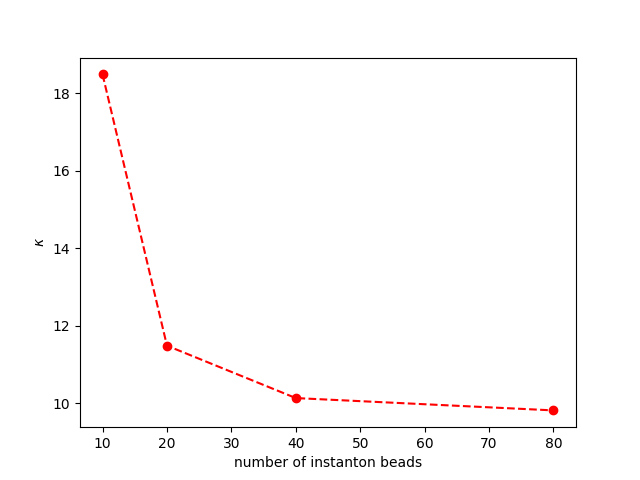
In this tutorial, the number of beads used in the example is much more than necessary. Please try the instanton calculation with 10 or 20 beads, and see how the results \(\kappa\) compare.
kappadat = np.array(
    [
        [10, 18.486247675370873],
        [20, 11.481103709870357],
        [40, 10.127813329699068],
        [80, 9.809437521247709],
    ]
)

plt.plot(kappadat[:, 0], kappadat[:, 1], "ro--")
plt.xlabel(r"number of instanton beads")
plt.ylabel(r"$\kappa$")
plt.show()
Total running time of the script: (1 minutes 10.482 seconds)