Phonon dispersions with unconstrained models and uncertainty quantification

Authors:

Paolo Pegolo @ppegolo Michele Ceriotti @ceriottm

Phonon dispersion curves are important experimental probes of the lattice dynamics of a material, and are commonly used to validate MLIPs. They are also crucial for computing temperature-dependent properties such as free energies and thermal conductivity.

Phonon bands are also used as a test of dynamical stability: a converged geometry optimization does not guarantee stability, as the structure may be a saddle point rather than a true minimum. A more telling test is the phonon dispersion: a stable structure has all real (positive) frequencies, while imaginary (negative) frequencies signal a dynamical instability, i.e. that a distortion of the structure (possibly accessible only for a larger cell) would lower the energy.

We consider three systems:

1. Al (FCC): a simple, stable metal. We show that constrained and unconstrained relaxations yield the same phonon dispersion when evaluated along the same \(\mathbf{q}\)-path—a subtlety that is important when using unconstrained models that do not fulfill exactly the symmetries of the system.

2. BaTiO₃ rhombohedral \(R3m\) (ferroelectric): the 0 K ground state discovered by unconstrained relaxation in the geometry relaxation recipe. All frequencies are real, confirming dynamical stability.

3. BaTiO₃ cubic \(Pm\bar{3}m\): the high-symmetry paraelectric structure, dynamically unstable with imaginary modes at \(\Gamma\) (ferroelectric soft mode).

This recipe also shows how to compute phonon band structures with uncertainty estimates from MLIP ensembles, using uqphonon, a wrapper around phonopy and i-PI. Uncertainty quantification is based on the construction of a shallow ensemble (cf. Kellner and Ceriotti, 2024), with the committee members obtained using the last-layer prediction rigidity framework (LLPR, Bigi et al., 2024; see also the PET-MAD UQ recipe).

import warnings

import numpy as np
import matplotlib.pyplot as plt
from matplotlib.patches import Patch
from ase import Atoms
from ase.build import bulk
from ase.constraints import FixSymmetry
from ase.filters import FrechetCellFilter
from ase.optimize import LBFGS
from pathlib import Path
import tempfile

import spglib
import upet
from upet.calculator import UPETCalculator
from phonopy import Phonopy
from phonopy.structure.atoms import PhonopyAtoms

# helper functions from uqphonon
from uqphonon import PhononEnsemble
from uqphonon._core import _phonopy_to_ase
from uqphonon._core import _resolve_bandpath
from uqphonon._plot import plot_bands

# Suppress warnings about matrix logarithm accuracy issued by scipy during geometry
# optimization to avoid cluttering the output
warnings.filterwarnings(
    "ignore",
    category=RuntimeWarning,
    message="logm result may be inaccurate, approximate err",
)

# sphinx_gallery_thumbnail_number = 3

Setup

We use the extra-small (XS) variant of PET-MAD v1.5.0. For production calculations, the S model would be a more accurate choice.

FMAX = 1e-4  # eV/Å, force convergence threshold
STEPS = 500  # max optimization steps
DELTA = 0.05  # Å, displacement amplitude for force constants
DEVICE = "cpu"

MODEL_BASE = "pet-mad"
MODEL_SIZE = "xs"
MODEL_VERSION = "1.5.0"
MODEL_NAME = f"{MODEL_BASE}-{MODEL_SIZE}"

calc = UPETCalculator(
    model=MODEL_NAME,
    device=DEVICE,
    dtype="float32",
    version=MODEL_VERSION,
)

Export model

uqphonon drives force evaluations through i-PI, which requires a TorchScript-exported metatomic model.

model_path = "model.pt"
upet.save_upet(
    model=MODEL_BASE,
    size=MODEL_SIZE,
    version=MODEL_VERSION,
    output=model_path,
)
print(f"Model saved to {model_path}")

Model saved to model.pt

Helpers

def report_symmetry(atoms, label=""):
    """Detect and report space group using spglib."""
    spglib_cell = (
        atoms.get_cell(),
        atoms.get_scaled_positions(),
        atoms.get_atomic_numbers(),
    )
    sg_loose = spglib.get_spacegroup(spglib_cell, symprec=1e-2)
    sg_tight = spglib.get_spacegroup(spglib_cell, symprec=1e-6)
    print(
        f"{label:30s}  loose (1e-2): {str(sg_loose):15s}  tight (1e-6): {str(sg_tight)}"
    )


def compute_phonons(
    atoms, model_path, supercell, bands=None, npoints=50, labels=None, label=""
):
    """Compute phonon band structure with phonopy and the ASE calculator."""
    print(f"\n--- {label} ---")

    phonopy_atoms = PhonopyAtoms(
        symbols=atoms.get_chemical_symbols(),
        cell=atoms.cell[:],
        scaled_positions=atoms.get_scaled_positions(),
    )

    phonon = Phonopy(
        phonopy_atoms,
        supercell_matrix=np.diag(supercell),
        primitive_matrix=np.eye(3),
    )
    phonon.generate_displacements(distance=DELTA)

    supercells = phonon.supercells_with_displacements
    forces = []
    for sc in supercells:
        sc_ase = Atoms(
            symbols=sc.symbols,
            cell=sc.cell,
            scaled_positions=sc.scaled_positions,
            pbc=True,
        )
        sc_ase.calc = atoms.calc
        forces.append(sc_ase.get_forces())

    phonon.forces = np.array(forces)
    phonon.produce_force_constants()
    phonon.symmetrize_force_constants()

    n_disp = len(supercells)
    n_atoms = len(supercells[0])
    print(f"{n_disp} displacements, {n_atoms} atoms/cell")

    # Resolve the band path using the same logic as uqphonon
    prim_atoms = _phonopy_to_ase(phonon.primitive)
    qpoints, connections, resolved_labels = _resolve_bandpath(
        prim_atoms, bands, npoints, labels=labels
    )
    phonon.run_band_structure(
        qpoints, path_connections=connections, labels=resolved_labels
    )

    # Wrap in a simple namespace so that .plot() and .compute_bands() work
    # like PhononEnsemble
    class _PhononResult:
        def __init__(self, ph):
            self._phonon = ph

        def plot(self, ax=None, mode="ensemble", unit="cm-1", **kwargs):
            return plot_bands(
                [self._phonon], self._phonon, mode=mode, unit=unit, ax=ax, **kwargs
            )

        def compute_bands(self, bandpath=None, npoints=151, labels=None):
            qpts, conns, lbls = _resolve_bandpath(
                prim_atoms, bandpath, npoints, labels=labels
            )
            self._phonon.run_band_structure(qpts, path_connections=conns, labels=lbls)

    return _PhononResult(phonon)


def compute_phonons_with_uq(
    atoms, model_path, supercell, bands=None, npoints=50, labels=None, label=""
):
    """Compute phonon band structure with uqphonon ensemble."""
    print(f"\n--- {label} ---")

    ensemble = PhononEnsemble(
        atoms,
        supercell_matrix=np.diag(supercell),
        model=str(model_path),
        device=DEVICE,
        primitive_matrix=np.eye(3),
    )
    ensemble.compute_displacements(distance=DELTA)

    workdir = Path(tempfile.gettempdir()) / f"uqphonon_{label.replace(' ', '_')}"
    ensemble.run_forces(workdir=workdir)
    n_disp, n_ens, n_atoms, _ = ensemble.forces.shape
    print(f"{n_ens} ensemble members, {n_disp} displacements, {n_atoms} atoms/cell")

    if bands is not None:
        ensemble.compute_bands(bandpath=bands, npoints=npoints, labels=labels)
    else:
        ensemble.compute_bands(npoints=npoints)

    return ensemble

Al (FCC)

FCC aluminum is dynamically stable. We use it to illustrate a subtlety that is relevant when using an unconstrained model to find the minimum energy structure and compute the phonons: as already seen in the geometry relaxation recipe, unconstrained relaxation slightly breaks the \(Fm\bar{3}m\) symmetry, which causes automatic \(\mathbf{q}\)-path finders to detect a different (lower-symmetry) path. Therefore the band structure looks different, even though the underlying physics is the same.

Constrained relaxation

We first relax the cell with FixSymmetry to keep it at perfect FCC symmetry.

SUPERCELL_AL = (4, 4, 4)

atoms_al_const = bulk("Al", "fcc", a=4.05)
atoms_al_const.set_constraint(FixSymmetry(atoms_al_const))
atoms_al_const.calc = calc

opt_c = LBFGS(
    FrechetCellFilter(atoms_al_const, mask=[True] * 3 + [False] * 3), logfile=None
)
opt_c.run(fmax=FMAX, steps=STEPS)
report_symmetry(atoms_al_const, "Al FCC constrained")
atoms_al_const.set_constraint(None)

Al FCC constrained              loose (1e-2): Fm-3m (225)      tight (1e-6): Fm-3m (225)

Unconstrained relaxation

Because of the small symmetry breaking, unconstrained relaxation converges to a slightly distorted cell with lower symmetry.

atoms_al_unconst = bulk("Al", "fcc", a=4.05)
atoms_al_unconst.calc = calc

opt_u = LBFGS(FrechetCellFilter(atoms_al_unconst), logfile=None)
opt_u.run(fmax=FMAX, steps=STEPS)
report_symmetry(atoms_al_unconst, "Al FCC unconstrained")

Al FCC unconstrained            loose (1e-2): Fm-3m (225)      tight (1e-6): P-1 (2)

Phonons with automatic q-path

Because the unconstrained cell has slightly broken symmetry, the automatically chosen path is that for \(P\bar{1}\) rather than the standard FCC path that is computed for the constrained optimization.

phonons_al_const_auto = compute_phonons(
    atoms_al_const,
    model_path,
    supercell=SUPERCELL_AL,
    label="Al constrained (auto)",
)

phonons_al_unconst_auto = compute_phonons(
    atoms_al_unconst,
    model_path,
    supercell=SUPERCELL_AL,
    label="Al unconstrained (auto)",
)

fig, (ax1, ax2) = plt.subplots(1, 2, figsize=(12, 5))

phonons_al_const_auto.plot(
    ax=ax1, mode="mean", unit="THz", color="tab:blue", std_alpha=0.2
)
ax1.set_title("Al (FCC), constrained")

phonons_al_unconst_auto.plot(
    ax=ax2, mode="mean", unit="THz", color="tab:red", std_alpha=0.2
)
ax2.set_title("Al (FCC), unconstrained")

plt.tight_layout()
plt.show()

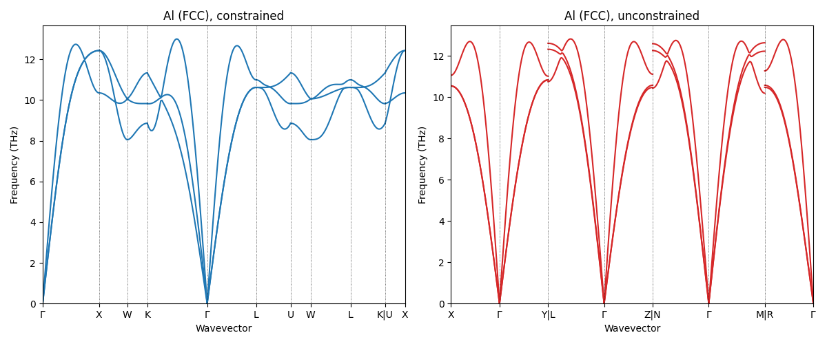
--- Al constrained (auto) ---
1 displacements, 64 atoms/cell

--- Al unconstrained (auto) ---
3 displacements, 64 atoms/cell

Phonons with explicit FCC q-path

The two plots look different. To confirm that the physics is the same, we repeat the calculation on both structures using the standard FCC path.

G = np.array([0.0, 0.0, 0.0])
X = np.array([0.5, 0.0, 0.5])
W = np.array([0.5, 0.25, 0.75])
K_fcc = np.array([0.375, 0.375, 0.75])
L = np.array([0.5, 0.5, 0.5])


def get_band(q_start, q_stop, N):
    return np.array([q_start + (q_stop - q_start) * i / (N - 1) for i in range(N)])


N_KPOINTS = 50

BANDS_FCC = [
    get_band(G, X, N_KPOINTS),
    get_band(X, W, N_KPOINTS),
    get_band(W, K_fcc, N_KPOINTS),
    get_band(K_fcc, G, N_KPOINTS),
    get_band(G, L, N_KPOINTS),
]

LABELS_FCC = ["$\\Gamma$", "X", "W", "K", "$\\Gamma$", "L"]

The force constants are already computed, so we only need to Fourier-interpolate along the new path.

phonons_al_const_auto.compute_bands(
    bandpath=BANDS_FCC, npoints=N_KPOINTS, labels=LABELS_FCC
)
phonons_al_unconst_auto.compute_bands(
    bandpath=BANDS_FCC, npoints=N_KPOINTS, labels=LABELS_FCC
)

fig, ax = plt.subplots(figsize=(8, 5))

phonons_al_const_auto.plot(
    ax=ax, mode="mean", unit="THz", color="tab:blue", std_alpha=0.2
)
phonons_al_unconst_auto.plot(
    ax=ax, mode="mean", unit="THz", color="tab:red", std_alpha=0.2
)

legend_elements = [
    Patch(facecolor="tab:blue", alpha=0.5, label="Constrained"),
    Patch(facecolor="tab:red", alpha=0.5, label="Unconstrained"),
]
ax.legend(handles=legend_elements, fontsize=11, loc="upper right")
ax.set_title("Al (FCC)")

plt.tight_layout()
plt.show()

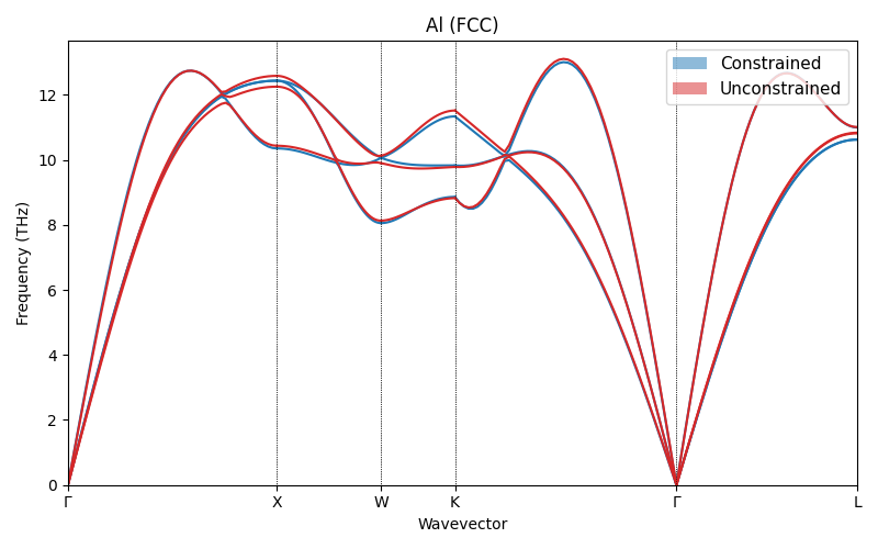
On the same \(\mathbf{q}\)-path, the two dispersions almost overlap. The apparent discrepancy from the automatic path comparison was due to the different reciprocal-space trajectories, not to physical difference. In practice the safest workflow is to perform a constrained relaxation, or to use spglib.standardize_cell to symmetrize the relaxed cell.

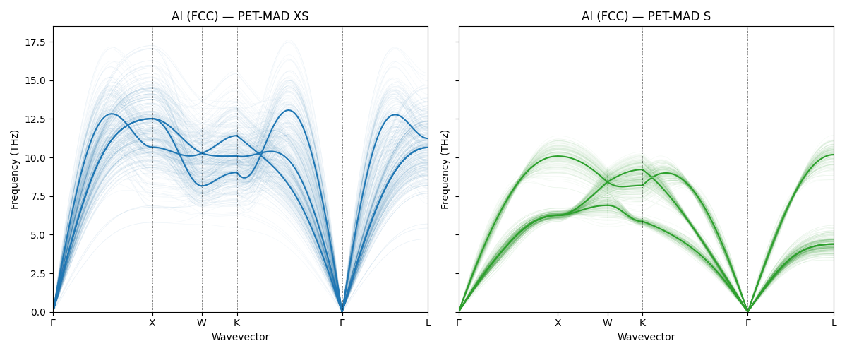
Phonons with uncertainty quantification

The phonon calculations above used a single model prediction for the forces. To assess the model’s confidence we can use an ensemble of predictions, comparing the XS and S variants of PET-MAD. The S model is more accurate but slower; the uncertainty bands show where predictions are reliable.

model_path_s = "model_s.pt"
upet.save_upet(
    model=MODEL_BASE,
    size="s",
    version=MODEL_VERSION,
    output=model_path_s,
)

ensemble_al_xs = compute_phonons_with_uq(
    atoms_al_const,
    model_path,
    supercell=SUPERCELL_AL,
    bands=BANDS_FCC,
    labels=LABELS_FCC,
    npoints=N_KPOINTS,
    label="Al XS (UQ)",
)

ensemble_al_s = compute_phonons_with_uq(
    atoms_al_const,
    model_path_s,
    supercell=SUPERCELL_AL,
    bands=BANDS_FCC,
    labels=LABELS_FCC,
    npoints=N_KPOINTS,
    label="Al S (UQ)",
)

--- Al XS (UQ) ---
128 ensemble members, 1 displacements, 64 atoms/cell

--- Al S (UQ) ---
128 ensemble members, 1 displacements, 64 atoms/cell

fig, (ax1, ax2) = plt.subplots(1, 2, figsize=(12, 5), sharey=True)

ensemble_al_xs.plot(
    ax=ax1, mode="ensemble", unit="THz", color="tab:blue", std_alpha=0.2
)
ax1.set_title("Al (FCC) — PET-MAD XS")

ensemble_al_s.plot(
    ax=ax2, mode="ensemble", unit="THz", color="tab:green", std_alpha=0.2
)
ax2.set_title("Al (FCC) — PET-MAD S")

plt.tight_layout()
plt.show()

BaTiO\(_3\) (\(R3m\))

As shown in the geometry relaxation recipe, unconstrained relaxation of cubic BaTiO\(_3\) converges to the ferroelectric \(R3m\) phase. Here we verify that it is dynamically stable.

We follow the workflow from the relaxation recipe: unconstrained relaxation, symmetry identification with spglib, cell standardization, and re-relaxation with FixSymmetry to obtain a clean \(R3m\) primitive cell for the phonon calculation.

A (2,2,2) supercell is used here to keep the example fast; larger supercells [e.g., (6,6,6)] would give better-converged dispersions.

SUPERCELL_BTO = (2, 2, 2)

a_bto = 4.00
bto_cubic = Atoms(
    symbols="BaTiO3",
    scaled_positions=[
        [0.0, 0.0, 0.0],  # Ba
        [0.5, 0.5, 0.5],  # Ti
        [0.5, 0.5, 0.0],  # O1
        [0.5, 0.0, 0.5],  # O2
        [0.0, 0.5, 0.5],  # O3
    ],
    cell=[a_bto, a_bto, a_bto],
    pbc=True,
)

Geometry optimization and symmetry constraints

We first relax the structure without constraints, to find the ferroelectric ground state.

bto_ferroelectric = bto_cubic.copy()
bto_ferroelectric.calc = calc

opt_ferro = LBFGS(FrechetCellFilter(bto_ferroelectric), logfile=None)
opt_ferro.run(fmax=FMAX, steps=STEPS)
report_symmetry(bto_ferroelectric, "BTO unconstrained")

/home/runner/work/atomistic-cookbook/atomistic-cookbook/.nox/pet-phonons/lib/python3.12/site-packages/upet/calculator.py:227: UserWarning: Some of the atomic energy uncertainties are larger than the threshold of 0.1 eV. The prediction is above the threshold for atoms [1].
  self.calculator.calculate(atoms, properties, system_changes)
BTO unconstrained               loose (1e-2): P1 (1)           tight (1e-6): P1 (1)

Scan spglib tolerance to identify the symmetry plateau (the range of tolerances over which spglib consistently reports the same space group).

spglib_cell = (
    bto_ferroelectric.get_cell(),
    bto_ferroelectric.get_scaled_positions(),
    bto_ferroelectric.get_atomic_numbers(),
)
for symprec in np.logspace(-3, np.log10(0.2), 10):
    res = spglib.get_spacegroup(spglib_cell, symprec=symprec)
    print(f"  symprec={symprec:.4f}  {res}")

symprec=0.0010  P1 (1)
symprec=0.0018  P1 (1)
symprec=0.0032  P1 (1)
symprec=0.0058  P1 (1)
symprec=0.0105  P1 (1)
symprec=0.0190  P1 (1)
symprec=0.0342  Cm (8)
symprec=0.0616  R3m (160)
symprec=0.1110  R3m (160)
symprec=0.2000  Pm-3m (221)

The relaxed cell still carries numerical noise that breaks exact \(R3m\) symmetry. We use standardize_cell to snap it onto ideal Wyckoff positions …

std_data = spglib.standardize_cell(spglib_cell, to_primitive=True, symprec=0.05)

bto_r3m = Atoms(
    numbers=std_data[2],
    scaled_positions=std_data[1],
    cell=std_data[0],
    pbc=True,
)

report_symmetry(bto_r3m, "BTO R3m (spglib)")

BTO R3m (spglib)                loose (1e-2): R3m (160)        tight (1e-6): R3m (160)

… and then we re-relax with FixSymmetry to get a clean \(R3m\) cell with zero forces and stresses, which is ideal for phonon calculations.

bto_r3m.set_constraint(FixSymmetry(bto_r3m))
bto_r3m.calc = calc

opt_r3m = LBFGS(FrechetCellFilter(bto_r3m, mask=[True] * 3 + [False] * 3), logfile=None)
opt_r3m.run(fmax=FMAX, steps=STEPS)
report_symmetry(bto_r3m, "BTO R3m (re-relaxed)")

bto_r3m.set_constraint(None)

BTO R3m (re-relaxed)            loose (1e-2): R3m (160)        tight (1e-6): R3m (160)

Phonon dispersion

We compute the phonon dispersion with the XS model, to verify the stability of the R3m phase.

ensemble_ferro = compute_phonons(
    bto_r3m,
    model_path,
    supercell=SUPERCELL_BTO,
    label="BTO R3m",
)

--- BTO R3m ---
/home/runner/work/atomistic-cookbook/atomistic-cookbook/.nox/pet-phonons/lib/python3.12/site-packages/upet/calculator.py:227: UserWarning: Some of the atomic energy uncertainties are larger than the threshold of 0.1 eV. The prediction is above the threshold for atoms [ 8  9 10 11 12 13 14 15].
  self.calculator.calculate(atoms, properties, system_changes)
8 displacements, 40 atoms/cell

fig, ax = plt.subplots(figsize=(10, 5))

ensemble_ferro.plot(
    ax=ax,
    mode="ensemble",
    unit="THz",
    color="tab:green",
    std_alpha=0.2,
)

ax.set_title(r"BaTiO$_3$ ($R3m$)")

plt.tight_layout()
plt.show()

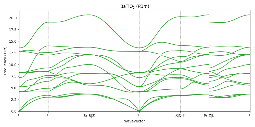
All phonon branches are positive across the Brillouin zone, confirming that the \(R3m\) phase is stable.

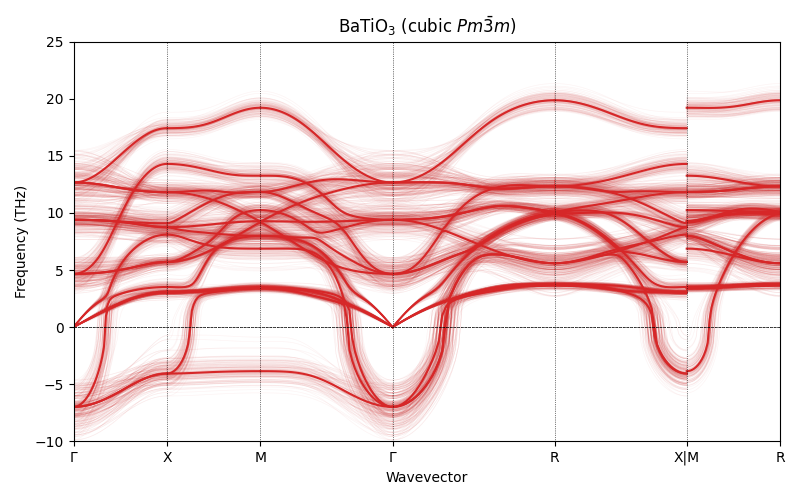
BaTiO\(_3\) (cubic \(Pm\bar{3}m\))

The cubic perovskite is the high-symmetry paraelectric structure. At 0 K we expect it to be dynamically unstable, with imaginary phonon modes at \(\Gamma\) corresponding to the ferroelectric soft mode that drives the \(Pm\bar{3}m \to R3m\) transition.

We relax the cubic cell with FixSymmetry to keep it at \(Pm\bar{3}m\).

bto_cubic_relax = bto_cubic.copy()
bto_cubic_relax.set_constraint(FixSymmetry(bto_cubic_relax))
bto_cubic_relax.calc = calc

opt_cubic = LBFGS(
    FrechetCellFilter(bto_cubic_relax, mask=[True] * 3 + [False] * 3), logfile=None
)
opt_cubic.run(fmax=FMAX, steps=STEPS)
report_symmetry(bto_cubic_relax, "BTO cubic (relaxed)")

bto_cubic_relax.set_constraint(None)

/home/runner/work/atomistic-cookbook/atomistic-cookbook/.nox/pet-phonons/lib/python3.12/site-packages/upet/calculator.py:227: UserWarning: Some of the atomic energy uncertainties are larger than the threshold of 0.1 eV. The prediction is above the threshold for atoms [1].
  self.calculator.calculate(atoms, properties, system_changes)
BTO cubic (relaxed)             loose (1e-2): Pm-3m (221)      tight (1e-6): Pm-3m (221)

Phonon dispersion

We use the enseble mode of the model to generate phonon bands with uncertainty estimates.

ensemble_cubic = compute_phonons_with_uq(
    bto_cubic_relax,
    model_path,
    supercell=SUPERCELL_BTO,
    label="BTO cubic",
)


fig, ax = plt.subplots(figsize=(8, 5))

ensemble_cubic.plot(
    ax=ax,
    mode="ensemble",
    unit="THz",
    color="tab:red",
    std_alpha=0.2,
)

ax.set_title(r"BaTiO$_3$ (cubic $Pm\bar{3}m$)")
ax.axhline(0, color="k", linestyle="--", linewidth=0.5)
ax.set_ylim(-10, 25)

plt.tight_layout()
plt.show()

--- BTO cubic ---
128 ensemble members, 3 displacements, 40 atoms/cell

Clear imaginary frequencies appear at \(\Gamma\), the ferroelectric soft mode. The uncertainty bands are well below the magnitude of the instability, confirming it is a genuine prediction of the model.

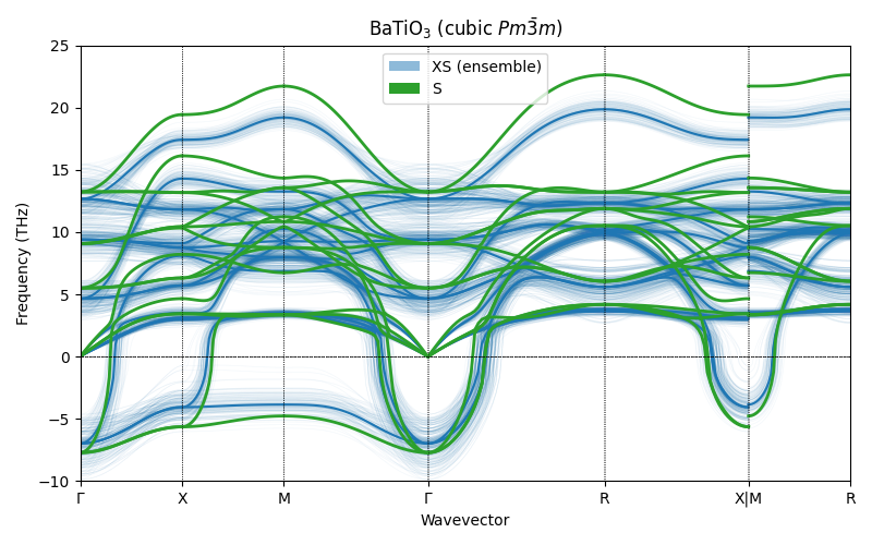
Validation with PET-MAD S

As a final check, we compute the cubic BaTiO₃ phonon dispersion with the larger PET-MAD S model (single prediction, no UQ) and overlay it on the XS ensemble bands. The cubic cell is re-relaxed with the S model before computing phonons, so the force constants are evaluated at the S model’s own (constrained) equilibrium.

calc_s = UPETCalculator(
    model="pet-mad-s",
    device=DEVICE,
    dtype="float32",
    version=MODEL_VERSION,
)

bto_cubic_s = bto_cubic.copy()
bto_cubic_s.set_constraint(FixSymmetry(bto_cubic_s))
bto_cubic_s.calc = calc_s

opt_cubic_s = LBFGS(
    FrechetCellFilter(bto_cubic_s, mask=[True] * 3 + [False] * 3), logfile=None
)
opt_cubic_s.run(fmax=FMAX, steps=STEPS)
report_symmetry(bto_cubic_s, "BTO cubic (S, re-relaxed)")
bto_cubic_s.set_constraint(None)

phonons_cubic_s = compute_phonons(
    bto_cubic_s,
    model_path_s,
    supercell=SUPERCELL_BTO,
    label="BTO cubic (S)",
)

BTO cubic (S, re-relaxed)       loose (1e-2): Pm-3m (221)      tight (1e-6): Pm-3m (221)

--- BTO cubic (S) ---
3 displacements, 40 atoms/cell

fig, ax = plt.subplots(figsize=(8, 5))

ensemble_cubic.plot(
    ax=ax, mode="ensemble", unit="THz", color="tab:blue", std_alpha=0.15
)
phonons_cubic_s.plot(
    ax=ax, mode="mean", unit="THz", color="tab:green", mean_linewidth=2.0
)
ax.set_title(r"BaTiO$_3$ (cubic $Pm\bar{3}m$)")
ax.axhline(0, color="k", linestyle="--", linewidth=0.5)
ax.set_ylim(-10, 25)
legend_elements = [
    Patch(facecolor="tab:blue", alpha=0.5, label="XS (ensemble)"),
    Patch(facecolor="tab:green", alpha=1.0, label="S"),
]
ax.legend(handles=legend_elements, fontsize=10)

plt.tight_layout()
plt.show()

/home/runner/work/atomistic-cookbook/atomistic-cookbook/examples/pet-phonons/pet-phonons.py:693: UserWarning: Creating legend with loc="best" can be slow with large amounts of data.
  plt.tight_layout()

The S model (green) falls within the XS ensemble bands, confirming that the XS uncertainty estimates are well-calibrated and that both models agree on the ferroelectric instability in cubic \(Pm\bar{3}m\).