A Guide to PET-MAD-DOS: Model Inference and Fine-Tuning

Authors:

How Wei Bin @HowWeiBin

This tutorial describes two ways in which one can use PET-MAD-DOS to predict the electronic density of states (DOS) of a structure:

1. Treating PET-MAD-DOS as a universal model: using the upet package, we will obtain high quality DOS predictions out of the box for a structure of interest.

2. Treating PET-MAD-DOS as a foundation model: we will illustrate how one can use the metatrain package to fine-tune the PET-MAD-DOS model for a specific application.

In the process, we will also go through the necessary data processing pipeline, starting from basic DFT outputs.

First, let’s begin by importing the necessary packages and helper functions

# sphinx_gallery_thumbnail_number = 2

from upet.calculator import PETMADDOSCalculator
import ase
import ase.io
import matplotlib.pyplot as plt
import numpy as np
import torch
import urllib.request
import os
import subprocess

Using PET-MAD-DOS out of the box

In this section, we are going to treat PET-MAD-DOS as a universal model and use it out-of-the-box to obtain predictions of the DOS for a sample of structures.

Step 1: Loading Sample Structures

We will start by loading a sample of structures, along with their associated DOS and mask. These are 5 structures from the training dataset used in the original PET-MAD-DOS publication.

# Load the structures
structs = ase.io.read("data/MAD_sample_structures.xyz", ":")

# Extract the DOS and mask
true_DOS = np.stack([s.info["DOS"] for s in structs])
true_mask = np.stack([s.info["mask"] for s in structs])
print(f"The shape of true_DOS is: {true_DOS.shape}")
print(f"The shape of true_mask is: {true_mask.shape}")

# Define the energy grid for the DOS
lower_bound, upper_bound = -148.1456 - 1.5, 79.1528 + 1.5
interval = 0.05
true_energy_grid = np.arange(lower_bound, upper_bound, interval)
print(f"The shape of true_energy_grid is: {true_energy_grid.shape}")

The shape of true_DOS is: (5, 4606)
The shape of true_mask is: (5, 4606)
The shape of true_energy_grid is: (4606,)

The true DOS is computed based on eigenvalues obtained from DFT calculations and projected on an energy grid (true_energy_grid) of size 4606. However, due to eigenvalue truncation in the dataset, the DOS is not necessarily well-defined at every point on the energy grid. For instance, if the highest computed eigenvalue of a structure A is at 3eV, the computed DOS would indicate that there are no states past 3 eV. However, that is false and is merely an artifact of eigenvalue truncation. Hence, an additional mask is included for each structure to show the regions where the DOS is well-defined. The DOS is considered well-defined up to 0.9eV below the minimum energy of the highest band in the DFT calculation. Following, we plot an example DOS together with its mask.

i_struct = 0  # index of the structure to visualize

# Plot DOS of the structure
plt.plot(true_energy_grid, true_DOS[i_struct], label="DFT DOS", color="red")
# Plot mask for the structure (multiplied by 10 for better visualization)
plt.plot(
    true_energy_grid,
    true_mask[i_struct] * 10,
    label="Mask x 10",
    linestyle="--",
    color="black",
)
plt.xlim(-60, 20)
plt.tick_params(axis="both", which="major", labelsize=14, width=2, length=6)
plt.xlabel(r"Energy - $\mathrm{E_F}$ [eV]", size=16)
plt.ylabel(r"DOS [$\mathrm{states}/eV$]", size=16)
plt.legend(fontsize=16)
plt.tight_layout()
plt.show()

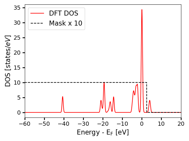
In this plot, the DOS is aligned such that the Fermi level is at 0eV. DOS values where the mask is 0 should not be considered reliable and should be ignored when comparing both spectra.

Step 2: Loading PET-MAD-DOS

Here we will load the PET-MAD-DOS model using the upet package and use it to predict the DOS. Although the target has size 4606 as seen in the cells above, in order to accomodate the energy reference agnostic loss function, PET-MAD-DOS predicts on a larger energy grid (energies) of size 4806.

# Load the calculator
pet_mad_dos_calculator = PETMADDOSCalculator(version="latest", device="cpu")

# Generate predictions for structures
energies, pred_DOS = pet_mad_dos_calculator.calculate_dos(structs)

print(f"The shape of pred_DOS is: {pred_DOS.shape}")
print(f"The shape of energies is: {energies.shape}")

Warning: You are sending unauthenticated requests to the HF Hub. Please set a HF_TOKEN to enable higher rate limits and faster downloads.
WARNING:huggingface_hub.utils._http:Warning: You are sending unauthenticated requests to the HF Hub. Please set a HF_TOKEN to enable higher rate limits and faster downloads.
/home/runner/work/atomistic-cookbook/atomistic-cookbook/.nox/pet-mad-dos/lib/python3.12/site-packages/metatomic/torch/ase_calculator.py:1482: UserWarning: `compute_requested_neighbors_from_options` is deprecated and will be removed in a future version. Please use `neighbor_lists_for_model` to get the calculators and call them directly.
  vesin.metatomic.compute_requested_neighbors_from_options(
The shape of pred_DOS is: torch.Size([5, 4806])
The shape of energies is: torch.Size([4806])

Step 3: Visualize the predictions

We can plot the predicted DOS and the true DOS on the same plot to see how they compare.

# Visualize the predictions and the true DOS on the same plot
plt.plot(energies, pred_DOS[i_struct], label="Predicted DOS", color="blue")
plt.plot(
    true_energy_grid, true_DOS[i_struct], label="DFT DOS", linestyle="--", color="red"
)

plt.xlim(-60, 20)
plt.tick_params(axis="both", which="major", labelsize=14, width=2, length=6)
plt.xlabel(r"Energy - $\mathrm{E_F}$ [eV]", size=16)
plt.ylabel(r"DOS [$\mathrm{states}/eV$]", size=16)
plt.legend(fontsize=16)
plt.tight_layout()
plt.show()

The profiles are very similar, but they are not aligned. This is because the energy reference is not well-defined. For this reason, during training of the model, the predictions are shifted to minimize the error with respect to the true DOS. Therefore, to compare the predicted DOS with the target, we need to do the same procedure.

# Define a function that minimizes the RMSE between the predicted and true DOS
# by shifting the energy axis
def get_dynamic_shift_agnostic_mse(predictions, targets, cutoff_mask):
    if predictions.shape[1] < targets.shape[1]:
        smaller = predictions
        bigger = targets
    else:
        smaller = targets
        bigger = predictions

    bigger_unfolded = bigger.unfold(1, smaller.shape[1], 1)
    smaller_expanded = smaller[:, None, :]
    delta = smaller_expanded - bigger_unfolded
    dynamic_delta = delta * cutoff_mask.unsqueeze(dim=1)
    device = predictions.device
    losses = torch.sum(dynamic_delta * dynamic_delta, dim=2)
    front_tail = torch.cumsum(predictions**2, dim=1)
    shape_difference = predictions.shape[1] - targets.shape[1]
    additional_error = torch.hstack(
        [
            torch.zeros(len(predictions), device=device).reshape(-1, 1),
            front_tail[:, :shape_difference],
        ]
    )
    total_losses = losses + additional_error
    final_loss, shift = torch.min(total_losses, dim=1)
    result = torch.mean(final_loss)

    return result, shift


# Compute the optimal shift and the associated MSE
MSEs, shifts = get_dynamic_shift_agnostic_mse(
    pred_DOS, torch.tensor(true_DOS), torch.tensor(true_mask)
)


# Function that adjusts the true DOS and mask so that it is aligned to the
# predictions based on the optimal shift obtained above. This is useful for
# visualizing the predictions and the true DOS on the same plot.
def adjust_DOS_and_mask(target, mask, shift):
    adjusted_DOSes = []
    adjusted_mask = []
    for index, s in enumerate(shift):
        front_pad = torch.zeros(s)
        end_pad = torch.zeros(200 - s)  # 200 is because the dimensionality of
        # the prediction is 200 larger than
        # that of the target
        adjusted_DOSes.append(torch.hstack([front_pad, target[index], end_pad]))
        adjusted_mask.append(torch.hstack([front_pad, mask[index], end_pad]))
    return torch.vstack(adjusted_DOSes), torch.vstack(adjusted_mask)


# Adjust the DOS and mask based on the optimal shifts obtained above
adjusted_true_DOS, adjusted_true_mask = adjust_DOS_and_mask(
    torch.tensor(true_DOS), torch.tensor(true_mask), shifts
)

# Visualize the predictions and the true DOS on the same plot
plt.plot(energies, pred_DOS[i_struct], label="Predicted DOS", color="blue")

plt.plot(
    energies, adjusted_true_DOS[i_struct], label="DFT DOS", linestyle="--", color="red"
)

plt.plot(
    energies,
    adjusted_true_mask[i_struct] * 10,
    label="Mask x 10",
    linestyle="-.",
    color="black",
)

plt.xlim(-60, 20)
plt.tick_params(axis="both", which="major", labelsize=14, width=2, length=6)
plt.xlabel(r"Energy - $\mathrm{E_F}$ [eV]", size=16)
plt.ylabel(r"DOS [$\mathrm{states}/eV$]", size=16)
plt.legend(fontsize=16)
plt.tight_layout()
plt.show()

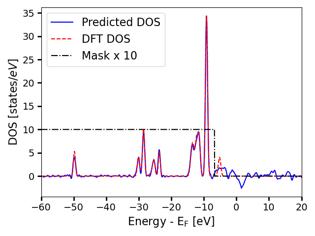
The alignment shows that the predicted DOS is actually very close to the true DOS for the region where the DOS values are physical, and essentially randomly oscillates after that point.

Step 4: Predicting the Bandgap

Additionally, PET-MAD-DOS comes with a CNN bandgap model that predicts the gap of a system based on the predicted DOS. Due to the inherent model noise and the high sensitivity of the bandgap to small errors in the DOS, obtaining the bandgap via a CNN model is more robust than deriving it from the predicted DOS.

pred_bandgap = pet_mad_dos_calculator.calculate_bandgap(structs, dos=pred_DOS)

true_bandgap = []
for i in structs:
    true_bandgap.append(i.info["gap"])
true_bandgap = torch.tensor(true_bandgap, dtype=torch.float32)

print(f"The predicted bandgaps are : {pred_bandgap}")
print(f"The DFT bandgaps are : {(true_bandgap)}")

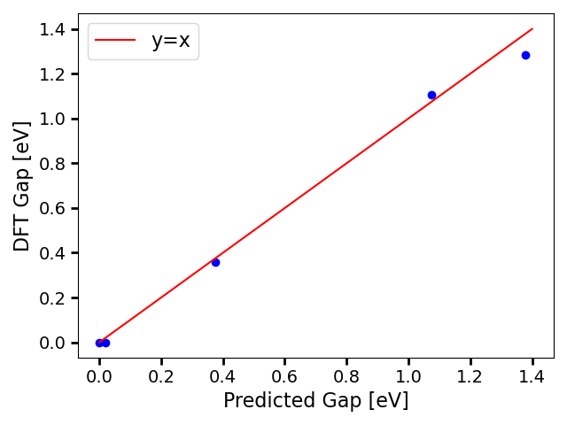
The predicted bandgaps are : tensor([0.0185, 1.0744, 0.3747, 1.3778, 0.0000])
The DFT bandgaps are : tensor([0.0000, 1.1067, 0.3567, 1.2842, 0.0000])

The band gaps show good agreement, following we generate a parity plot:

plt.scatter(pred_bandgap, true_bandgap, color="blue")
plt.plot([0, 1.4], [0, 1.4], label="y=x", color="red")
plt.tick_params(axis="both", which="major", labelsize=14, width=2, length=6)
plt.xlabel(r"Predicted Gap [eV]", size=16)
plt.ylabel(r"DFT Gap [eV]", size=16)
plt.legend(fontsize=16)
plt.tight_layout()
plt.show()

Finetuning PET-MAD-DOS on specific applications

In this section, we are going to treat PET-MAD-DOS as a foundation model and finetune it on a Gallium Arsenide (GaAs) system. We will first demonstrate the data processing pipeline starting from DFT outputs, and then we will show how to use the metatrain package to finetune the model.

Step 1: Data Processing

The following cells will show how to process a dataset containing eigenvalues to obtain the corresponding DOS and mask that can be used for fine-tuning PET-MAD-DOS. We will start by loading some GaAs sample structures containing eigenvalues and k-point weights from zenodo.

# The data processing pipeline uses the computed eigenvalues at each k-point,
# along with its associated k-point weight (where relevant) to generate the DOS
# and mask for each structure. The DOS is generated by applying gaussian
# broadening on each eigenenergy, and projected on an energy grid. For the
# purposes of fine-tuning, the energy grid will be identical to the one used for
# the training of PET-MAD-DOS.

url = "https://zenodo.org/records/19655792/files/GaAs_sample_structures.xyz?download=1"
filename = "GaAs_sample_structures.xyz"
urllib.request.urlretrieve(url, filename)
GaAs_sample_structures = ase.io.read("GaAs_sample_structures.xyz", ":")

Then define the function that will add the computed DOS and mask to the info of each structure.

def compute_structure_DOS_and_mask(
    structure: ase.Atoms, smearing: float, energy_grid: np.ndarray, n_extra_targets: int
):
    """Compute the DOS and mask for a structure based on its eigenvalues and k-points.

    The DOS is generated by applying gaussian broadening on each eigenenergy, and
    projected on an energy grid.

    The dos and mask are added to the info of the structure as "DOS" and "mask"
    respectively.

    :param structure: The input structure for which the DOS and mask will be computed.
       This should contain the info fields "eigvals" and "kweight" corresponding to
       the eigenvalues (n_kpoints, n_bands) and k-point weights (n_kpoints,) obtained
       from DFT calculations.
    :param smearing: The smearing value (in eV) to be used for gaussian broadening
       of the eigenenergies.
    :param energy_grid: The energy grid (in eV) on which the DOS will be projected.
    """
    eigenvalues = structure.info["eigvals"]  # shape (n_kpoints, n_bands)
    kweights = structure.info["kweight"]  # shape (n_kpoints,), sums to 2

    confident_energy_upper_bound = (
        np.min(eigenvalues[:, -1]) - 0.9
    )  # 0.9eV below the minimum of the highest band

    n_bands = eigenvalues.shape[1]

    # Flatten eigenvalues to shape (n_kpoints * n_bands,)
    eigenvalues = eigenvalues.flatten()
    # Ensure that the eigenvalues are mapped to the correct weight,
    # shape (n_kpoints * n_bands,)
    kweights = kweights.repeat(n_bands)

    # Compute the DOS on the energy grid by applying Gaussian broadening
    # on each eigenvalue
    delta_E = (energy_grid - eigenvalues[:, None]) / smearing
    gaussian_weights = np.exp(-0.5 * delta_E**2)
    normalization = 1 / np.sqrt(2 * np.pi * smearing**2)
    dos = (
        np.sum(kweights[:, None] * gaussian_weights, axis=0) * normalization
    )  # Apply Gaussian smearing and sum contributions

    # Define the mask
    mask = (energy_grid <= confident_energy_upper_bound).astype(int)

    # To prepare the data for fine-tuning, we will pad the DOS and mask with
    # zeros in front based on the number of extra targets that PET-MAD-DOS
    # predicts. These values will be ignored during loss computation.
    dos_padded = np.concatenate([np.zeros(n_extra_targets), dos])
    mask_padded = np.concatenate([np.zeros(n_extra_targets), mask])

    # Store the dos and mask in the structure info for training
    structure.info["DOS"] = dos_padded.astype(np.float32)
    structure.info["mask"] = mask_padded.astype(np.float32)

And apply it to each structure in the dataset.

# After defining the energy grid, we can now compute the DOS and the
# mask for each structure.
for struct in GaAs_sample_structures:
    compute_structure_DOS_and_mask(
        struct,
        # Same smearing value as the one used in the MAD training data
        smearing=0.3,
        # For fine-tuning, we will use the same energy grid as the one used for
        # training PET-MAD-DOS
        energy_grid=true_energy_grid,
        # PET-MAD-DOS predicts 200 more DOS
        # values per structure (4806 - 4606 = 200)
        n_extra_targets=200,
    )

# Store the processed structures as a new XYZ file for fine-tuning
# ase.io.write("GaAs_processed_structures.xyz", GaAs_sample_structures)

One would save the processed structures as a new XYZ file to to the fine-tuning, as demonstrated in the commented line. However, for the purposes of this tutorial, we will use datasets that have already been processed, as can be obtained from the MaterialsCloud archive. We just need to pad the DOS and mask with zeros in front to make the dimensionality compatible with the PET-MAD-DOS predictions.

# PET-MAD-DOS predicts 200 more DOS
# values per structure (4806 - 4606 = 200)
n_extra_targets = 200

GaAs_sample_train_structures = ase.io.read("data/GaAs_sample_train_structures.xyz", ":")
GaAs_sample_val_structures = ase.io.read("data/GaAs_sample_val_structures.xyz", ":")
GaAs_sample_test_structures = ase.io.read("data/GaAs_sample_test_structures.xyz", ":")


def pad_DOS(struct, n_extra_targets):
    dos_padded = np.concatenate([np.zeros(n_extra_targets), struct.info["DOS"]])
    mask_padded = np.concatenate([np.zeros(n_extra_targets), struct.info["mask"]])

    struct.info["trainingDOS"] = dos_padded
    struct.info["trainingmask"] = mask_padded


# To prepare the structures for training
for struct in GaAs_sample_train_structures:
    pad_DOS(struct, n_extra_targets)

for struct in GaAs_sample_val_structures:
    pad_DOS(struct, n_extra_targets)

for struct in GaAs_sample_test_structures:
    pad_DOS(struct, n_extra_targets)

ase.io.write("GaAs_processed_train.xyz", GaAs_sample_train_structures)
ase.io.write("GaAs_processed_val.xyz", GaAs_sample_val_structures)
ase.io.write("GaAs_processed_test.xyz", GaAs_sample_test_structures)

Step 2: Model Loading

Now we need to download the PET-MAD-DOS checkpoint and place it in the local directory so that it can be referenced in the metatrain YAML configuration files for fine-tuning.

# Download the checkpoint from Zenodo and copy it to the local directory
url = "https://zenodo.org/records/19655792/files/pet-mad-dos-v1.0.ckpt?download=1"

checkpoint_path = "pet-mad-dos-v1.0.ckpt"
if not os.path.exists(checkpoint_path):
    print("Downloading PET-MAD-DOS checkpoint...")
    urllib.request.urlretrieve(url, checkpoint_path)

Downloading PET-MAD-DOS checkpoint...

Step 3: Fine-tuning the model

Now we are ready to fine-tune the model using the metatrain package. We will use the mtt train command to train the model, alongside with a supporting YAML configuration file that specifies the training hyperparameters.

device: cpu
base_precision: 64
seed: 42

architecture:
  name: "pet"
  training:
    batch_size: 1
    num_epochs: 10
    learning_rate: 0.01
    atomic_baseline:
      mtt::dos: 0.0
    scale_targets: false
    loss:
      mtt::dos:
        type: masked_dos
        weight: 1.0
        grad_weight: 1e-4
        int_weight: 2
        extra_targets: 200  # Number of extra zero-padded targets to ignore during loss computation
        reduction: mean
    finetune:
      method: "full"
      read_from: pet-mad-dos-v1.0.ckpt

# Section defining the parameters for system and target data
training_set:
  systems: GaAs_processed_train.xyz
  targets:
    mtt::dos:
      key: trainingDOS
      per_atom: false
      type: scalar
      num_subtargets: 4806
  extra_data:
    mtt::dos_mask:
      key: trainingmask
      per_atom: false
      type: scalar
      num_subtargets: 4806

validation_set:
  systems: GaAs_processed_val.xyz
  targets:
    mtt::dos:
      key: trainingDOS
      per_atom: false
      type: scalar
      num_subtargets: 4806
  extra_data:
    mtt::dos_mask:
      key: trainingmask
      per_atom: false
      type: scalar
      num_subtargets: 4806

test_set: 0.0

# Begin finetuning
subprocess.run(
    ["mtt", "train", "finetune.yaml", "-o", "fine_tune-model.pt"], check=True
)

CompletedProcess(args=['mtt', 'train', 'finetune.yaml', '-o', 'fine_tune-model.pt'], returncode=0)

Step 4: Evaluating the model

After training, we can evaluate the model on the test set using the mtt eval command, alongside with a supporting YAML configuration file that specifies the evaluation hyperparameters.

systems: 
  read_from: ./GaAs_processed_test.xyz
targets:
  mtt::dos:
    key: trainingDOS
    per_atom: false
    type: scalar
    num_subtargets: 4806

subprocess.run(
    ["mtt", "eval", "fine_tune-model.pt", "eval.yaml", "-o", "pred.xyz"], check=True
)

output = ase.io.read("pred.xyz", ":")

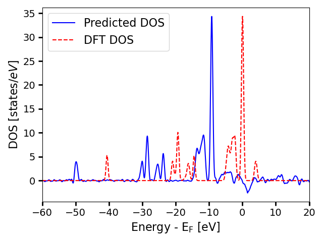
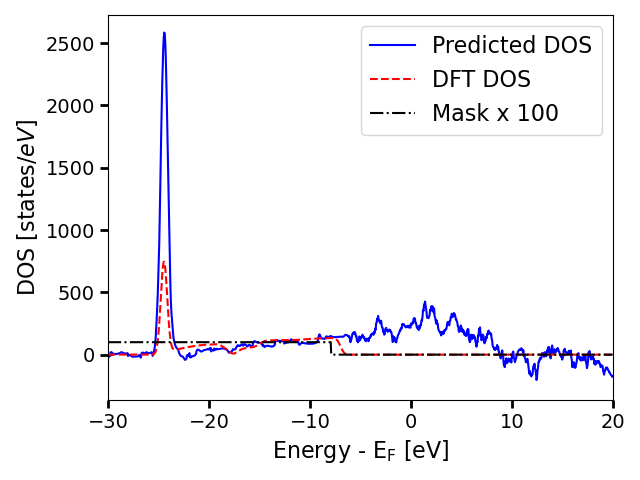
As we have only fine-tuned for 10 epochs on a tiny dataset, the model performance is not expected to be good. However, this simply serves as a demonstration of how to use the fine-tuned model.

predicted_DOS = []
for struct in output:
    predicted_DOS.append(struct.info["mtt::dos"])
predicted_DOS = torch.tensor(predicted_DOS)

true_DOS = []
true_mask = []
for struct in GaAs_sample_test_structures:
    true_DOS.append(struct.info["DOS"])
    true_mask.append(struct.info["mask"])
true_DOS = np.stack(true_DOS)
true_mask = np.stack(true_mask)

# Compute the optimal shift and the associated MSE
MSEs, shifts = get_dynamic_shift_agnostic_mse(
    predicted_DOS, torch.tensor(true_DOS), torch.tensor(true_mask)
)

# Adjust the DOS and mask based on the optimal shifts obtained above
adjusted_true_DOS, adjusted_true_mask = adjust_DOS_and_mask(
    torch.tensor(true_DOS), torch.tensor(true_mask), shifts
)

# Visualize the predictions and the true DOS on the same plot
i_struct = 0  # index of the structure to visualize

plt.plot(energies, predicted_DOS[i_struct], label="Predicted DOS", color="blue")

plt.plot(
    energies, adjusted_true_DOS[i_struct], label="DFT DOS", linestyle="--", color="red"
)

plt.plot(
    energies,
    adjusted_true_mask[i_struct] * 100,
    label="Mask x 100",
    linestyle="-.",
    color="black",
)

plt.xlim(-30, 20)
plt.tick_params(axis="both", which="major", labelsize=14, width=2, length=6)
plt.xlabel(r"Energy - $\mathrm{E_F}$ [eV]", size=16)
plt.ylabel(r"DOS [$\mathrm{states}/eV$]", size=16)
plt.legend(fontsize=16)
plt.tight_layout()
plt.show()

/home/runner/work/atomistic-cookbook/atomistic-cookbook/examples/pet-mad-dos/pet-mad-dos.py:483: UserWarning: Creating a tensor from a list of numpy.ndarrays is extremely slow. Please consider converting the list to a single numpy.ndarray with numpy.array() before converting to a tensor. (Triggered internally at /pytorch/torch/csrc/utils/tensor_new.cpp:253.)
  predicted_DOS = torch.tensor(predicted_DOS)