ML surrogate for the electron density and derived properties

Authors:

Joseph W. Abbott @jwa7

This recipe demonstrates how to predict the electron density of a molecule with a pretrained machine learning model and use the prediction for two purposes: (1) as an improved initial guess for a self-consistent field (SCF) calculation that reduces the number of iterations to convergence, and (2) as a direct source of electronic properties without running any further full SCF cycles.

The model is a PET (Point Edge Transformer) architecture trained with metatrain on the SCFBench dataset of PBE/def2-SVP density functional theory calculations on small organic molecules. It predicts the expansion coefficients of the electron density using an overlap-metric resolution-of-identity (RI) fit onto the def2-universal-jfit auxiliary basis, and the downstream DFT calculations are carried out with PySCF.

import os
import sys

import ase
import chemiscope
import matplotlib.pyplot as plt
import metatensor.torch as mts
import numpy as np
from IPython.display import HTML
from metatomic.torch import ModelOutput, load_atomistic_model
from metatomic.torch.ase_calculator import MetatomicCalculator
from pyscf import dft
from atomistic_cookbook_utils import download_with_retry

# Add data/ to sys.path so rho_utils can be imported directly.
# sphinx-gallery runs scripts via exec(), so __file__ is unavailable;
# the CWD is set to the example folder, so a relative path works.
_data_dir = os.path.abspath("data")
sys.path.insert(0, _data_dir)
from rho_utils import (  # noqa: E402
    atoms_to_pyscf,
    dm_from_ri_coefficients,
    nmae_percent,
    plot_density_slice,
    run_scf,
    visualise_density,
)

The density fitting (RI) approximation

Kohn-Sham DFT represents the electron density through the density matrix \(D_{\mu\nu}\),

\[\rho(\mathbf{r}) \;=\; \sum_{\mu\nu} D_{\mu\nu}\, \phi_\mu(\mathbf{r})\,\phi_\nu(\mathbf{r})\;,\]

where \(\{\phi_\mu\}\) are the contracted Gaussian orbital basis functions. The SCF cycle repeatedly builds the Fock matrix \(F[D] = h + V_J[D] + V_{xc}[D]\) and diagonalises it until \(D\) no longer changes.

The resolution-of-identity (RI) approximation re-expands the density on a compact, atom-centred auxiliary basis \(\{\chi_P\}\),

\[\tilde\rho(\mathbf{r}) \;=\; \sum_P c_P\,\chi_P(\mathbf{r})\;.\]

The coefficients \(\{c_P\}\) are found by minimising the squared pointwise error of the expansion,

\[\min_{\{c_P\}}\; \int [\rho(\mathbf{r}) - \tilde\rho(\mathbf{r})]^2\,\mathrm{d}\mathbf{r}\;.\]

This is the overlap-metric (or S-fit) variant of RI. The approximation is not exact for a finite auxiliary basis, but it has three properties that make \(\{c_P\}\) an attractive machine-learning target:

• Compact. A vector of \(N_\text{aux}\) numbers rather than an \(N_\text{ao}\times N_\text{ao}\) matrix.

• Local. The basis functions are atom-centred, so the coefficients naturally decompose by chemical environment and transfer across systems.

• Systematically improvable. Enlarging the auxiliary basis (essentially by tuning the \(L_\text{max}\) and number of onsite radial functions parameters) generally reduces the fitting error towards zero. This comes at increased cost, both in the fitting of the RI coefficients in data generation and in the training and inference of the resulting ML model. An additional caveat is that a larger auxiliary basis may also be more difficult to learn.

Given a predicted \(\tilde\rho\), two downstream workflows become cheaper:

• Accelerated SCF. Diagonalising the Fock matrix built from \(\tilde\rho\), \(F[\tilde\rho] = h + V_J[\tilde\rho] + V_{xc}[\tilde\rho]\), yields a density matrix \(D_0\) already close to self-consistency, reducing the number of SCF iterations needed.

• Downstream properties. Observables that can be derived from \(\rho\) – such as the electric dipole moment \(\boldsymbol{\mu} = -\int \mathbf{r}\,\rho(\mathbf{r})\, \mathrm{d}\mathbf{r}\) – can also be derived directly from \(\tilde\rho\) without running a full SCF cycle (though a diagonalization step may be required). The quality depends on how closely \(\tilde\rho\) approximates the true ground-state density.

System setup

We use a small organic molecule from the test set SCFBench dataset, a seven-atom \(\text{C}_2\text{H}_2\text{O}_3\) system computed at the PBE/def2-SVP level of theory, with RI decomposition onto the def2-universal-jfit auxiliary basis set. The DFT functional, orbital basis, and RI auxiliary basis are set to match the training data.

atoms = ase.Atoms(
    numbers=[8, 6, 6, 1, 8, 8, 1],
    positions=[
        [-1.3058, -1.0321, -1.0321],
        [-1.0843, -0.1924, -0.1924],
        [0.3229, 0.2412, 0.2412],
        [-1.8735, 0.3561, 0.3561],
        [0.4843, 1.0926, 1.0926],
        [1.3055, -0.4059, -0.4059],
        [2.1509, -0.0596, -0.0596],
    ],
)
atoms.center(about=atoms.get_center_of_mass())

BASIS = "def2-svp"  # DFT atomic orbital basis
XC = "pbe"  # XC functional
AUXBASIS = "def2-universal-jfit"  # auxiliary basis for the RI fit

# Visualize the molecule with chemiscope
chemiscope.show(
    atoms,
    mode="structure",
    settings=chemiscope.quick_settings(structure_settings={"rotation": True}),
)

×

×

Baseline: DFT from the SAD initial guess

PySCF’s default initial density matrix is the superposition of atomic densities (SAD): pre-computed atomic density matrices are stacked block-diagonally, ignoring all bonding. This is a reasonable but simple starting point. Other (and possibly better) initial guess schemes are available, but we only focus on the SAD here. We store this in dm_sad to compare with the RI reference and ML predictions below.

# Get and store the SAD initial guess DM
molecule = atoms_to_pyscf(atoms, BASIS)  # PySCF molecule object
mf_baseline = dft.RKS(molecule)  # initialize KS-DFT solver
mf_baseline.xc = XC  # set functional
dm_sad = mf_baseline.get_init_guess()  # SAD DM

# Run SCF with SAD initial guess and store the converged DM
mf_conv, n_sad = run_scf(atoms, XC, BASIS, dm0=dm_sad)
dm_conv = mf_conv.make_rdm1()

print(f"SAD initial guess → converged in {n_sad} cycles")
print(f"Converged SCF energy: {mf_conv.e_tot:.6f} Ha")

converged SCF energy = -302.531435204643
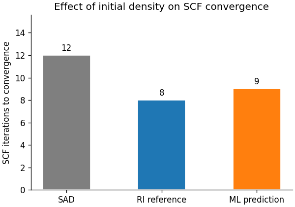
SAD initial guess → converged in 12 cycles
Converged SCF energy: -302.531435 Ha

RI reference coefficients

The reference coefficients from the SCFBench dataset for the example molecule are loaded below. They are stored in a TensorMap file (extension .mts). To reiterate, these are computed using the RI decomposition of the converged electron density, and represent the theoretical best that any ML model trained with this scheme can achieve for this auxiliary basis. Any errors in observables computed from the RI density relative to the true SCF density are a consequence of the incompleteness of the RI basis set.

The helper dm_from_ri_coefficients builds the Fock matrix \(F = h + V_J[\tilde\rho] + V_{xc}[\tilde\rho]\) from the RI coefficients, then diagonalises it to obtain a density matrix. This is (almost definitely) not a self-consistent density, but it is (hopefully) a good start. Indeed, running SCF with the RI reference initial guess reduces the number of iterations.

# Load the reference SCFBench RI coefficients for this molecule
ref_coefficients = mts.load(
    os.path.join(_data_dir, "scfbench_test_molecule_3464_rho_c_jfit.mts")
)

# Compute the density matrix from the RI coefficients, then run SCF with it as the
# initial guess
dm_ri = dm_from_ri_coefficients(atoms, ref_coefficients, XC, BASIS, AUXBASIS)
_, n_ri = run_scf(atoms, XC, BASIS, dm0=dm_ri)

print(f"RI reference initial guess → converged in {n_ri} cycles")

converged SCF energy = -302.531435204635
RI reference initial guess → converged in 8 cycles

ML-predicted RI coefficients

We now replace the reference coefficients with the output of the pretrained PET model. The model takes as input the atomic types and positions and returns a TensorMap of predicted RI coefficients with the same structure as the reference above – one block per \((\lambda, \sigma, Z)\) tuple of angular momentum, inversion parity, and atomic species.

This model has been trained on the whole SCFBench dataset of ~45k molecules, using an extension of the PET architecture for atomic basis targets.

# Download the pretrained model
download_with_retry(
    "https://github.com/ppegolo/labcosmo_ictp_school/raw/refs/heads/tmp/pet-density.pt",
    "model.pt",
)
model_path = "model.pt"

# Load the model as an ASE calculator
target_name = "mtt::rho_c_jfit_overlap"
model = load_atomistic_model(model_path)
calculator = MetatomicCalculator(model)

# Run inference on the model to predict RI coefficients for our example molecule
ml_coefficients = calculator.run_model(
    atoms, {target_name: ModelOutput(per_atom=True)}
)[target_name]

# Construct the ML initial guess density matrix from the predicted RI coefficients
dm_ml = dm_from_ri_coefficients(atoms, ml_coefficients, XC, BASIS, AUXBASIS)

# Run SCF with the ML initial guess
_, n_ml = run_scf(atoms, XC, BASIS, dm0=dm_ml)

print(f"ML initial guess → converged in {n_ml} cycles")

/home/runner/work/atomistic-cookbook/atomistic-cookbook/.nox/ml-density/lib/python3.11/site-packages/metatomic/torch/ase_calculator.py:1482: UserWarning: `compute_requested_neighbors_from_options` is deprecated and will be removed in a future version. Please use `neighbor_lists_for_model` to get the calculators and call them directly.
  vesin.metatomic.compute_requested_neighbors_from_options(
converged SCF energy = -302.531435204628
ML initial guess → converged in 9 cycles

SCF acceleration

Both the RI reference and the ML prediction reduce the SCF iteration count compared with the SAD baseline. The RI reference establishes the best achievable reduction for this auxiliary basis; the ML model reaches a similar reduction without ever having seen this molecule.

labels = ["SAD", "RI reference", "ML prediction"]
counts = [n_sad, n_ri, n_ml]
colors = ["C7", "C0", "C1"]

fig, ax = plt.subplots(figsize=(5, 3.5), constrained_layout=True, dpi=120)
bars = ax.bar(labels, counts, color=colors, edgecolor="white", width=0.5)
ax.bar_label(bars, padding=3, fontsize=10)
ax.set_ylabel("SCF iterations to convergence")
ax.set_title("Effect of initial density on SCF convergence")
ax.set_ylim(0, max(counts) * 1.3)
ax.spines[["top", "right"]].set_visible(False)

Visualize the electron density (in 3D)

The density matrix can be used to compute the electron density on a uniform real-space grid (a cube file) and visualized. The resolution of the grid is kept low for faster rendering.

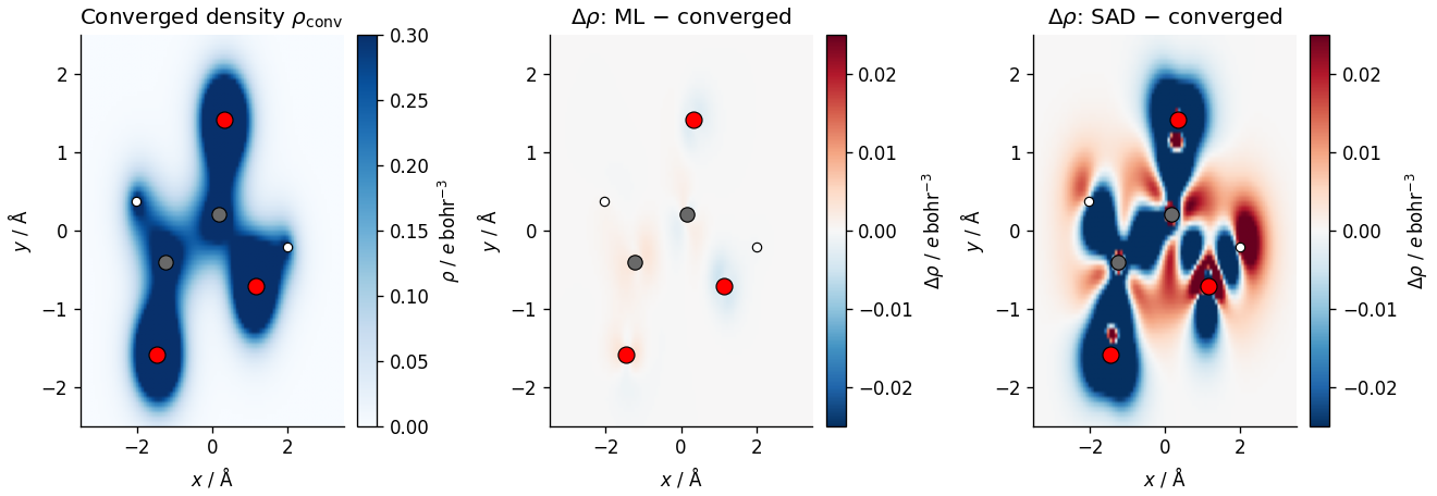
Here we plot the self consistent density, as well as the delta densities between this and the densities constructed from the i) SAD initial guess and ii) reference RI coefficients and iii) ML-predicted coefficients.

Note the isovalues used here for visual clarity, which also indicate the relative scales of the errors in the initial guesses. The SAD delta-density is large and structured, missing the redistribution of charge due to bonding. The ML prediction recovers the converged density far more accurately than the SAD guess. Residuals are small and featureless, and concentrated near the nuclear cores. However, there are still residual errors relative to the RI reference.

First the converged density

HTML(
    visualise_density(molecule, dm_conv, isoval=2e-3)  # SCF converged density
)

3Dmol.js failed to load for some reason. Please check your browser console for error messages.

Delta densities between the converged density and the SAD initial guess

HTML(
    visualise_density(molecule, dm_conv - dm_sad, isoval=1e-3)  # ∆ density - SAD
)

3Dmol.js failed to load for some reason. Please check your browser console for error messages.

Delta densities between the converged density and the RI reference initial guess

HTML(
    visualise_density(molecule, dm_conv - dm_ri, isoval=1e-4)  # ∆ density - RI
)

3Dmol.js failed to load for some reason. Please check your browser console for error messages.

Delta densities between the converged density and the ML predicted initial guess

HTML(
    visualise_density(molecule, dm_conv - dm_ml, isoval=1e-4)  # ∆ density - ML
)

3Dmol.js failed to load for some reason. Please check your browser console for error messages.

Visualizing the electron density (in 2D)

The 3D viewers above show isosurfaces. A complementary view is a 2D density slice through the molecular plane. Since all heavy atoms lie in the \(y = z\) plane, a 2D cut reveals the electron density profile in quantitative colour-mapped detail.

plot_density_slice(molecule, atoms, dm_conv, dm_ml, dm_sad)

<Figure size 1320x456 with 6 Axes>

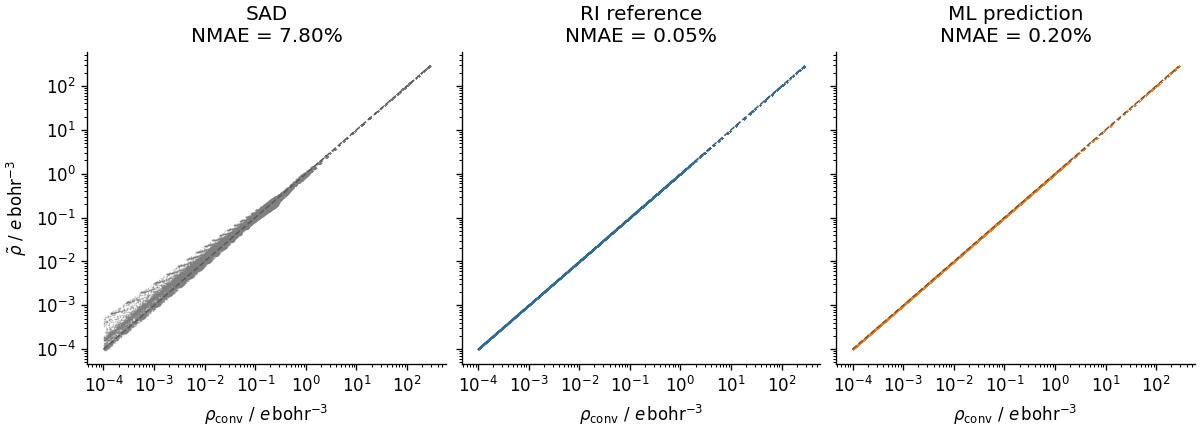
Density parity plots

For a quantitative comparison we evaluate each density on the DFT quadrature grid and plot the predicted value against the converged reference point-by-point. The normalised mean absolute error (NMAE) summarises the agreement over the whole grid with a single number, as is a common metric in density-learning literature.

\[\text{NMAE} \;=\; \frac{\int |\tilde\rho(\mathbf{r}) - \rho_\mathrm{conv}(\mathbf{r})| \,\mathrm{d}\mathbf{r}} {\int \rho_\mathrm{conv}(\mathbf{r})\,\mathrm{d}\mathbf{r}} \times 100\%\;.\]

The RI reference sets the achievable floor for this auxiliary basis; the ML prediction should approach it, while the SAD guess will be substantially worse.

# Evaluate AOs on the grid
grid_coords = mf_conv.grids.coords  # (npts, 3), Bohr
grid_weights = mf_conv.grids.weights  # (npts,)
ao_at_grid = molecule.eval_gto("GTOval_sph", grid_coords)  # (npts, nao)


def _dm_to_rho(dm):
    """ρ(r) = Σ_μν D_μν φ_μ(r) φ_ν(r) evaluated on the pre-built grid."""
    return np.einsum("pi,ij,pj->p", ao_at_grid, dm, ao_at_grid)


# Compute the reference (converged) real-space density
rho = _dm_to_rho(dm_conv)

fig, axes = plt.subplots(
    1, 3, figsize=(10, 3.6), constrained_layout=True, dpi=120, sharey=True
)

for ax, dm, color, label in [
    (axes[0], dm_sad, "C7", "SAD"),
    (axes[1], dm_ri, "C0", "RI reference"),
    (axes[2], dm_ml, "C1", "ML prediction"),
]:
    rho_guess = _dm_to_rho(dm)
    n_electrons = grid_weights @ rho_guess
    nmae = nmae_percent(rho_guess, rho, grid_weights)
    print(f"Electrons ({label}): {n_electrons:.6f}  (expected {molecule.nelectron})")
    print(f"NMAE% ({label}): {nmae:.6f}")

    ax.scatter(
        rho[
            rho > 1e-4
        ],  # only plot where the converged density is above a small threshold
        rho_guess[rho > 1e-4],
        s=0.8,
        alpha=0.25,
        color=color,
        rasterized=True,
        linewidths=0,
    )
    lo, hi = rho[rho > 1e-4].min(), rho[rho > 1e-4].max()
    ax.plot([lo, hi], [lo, hi], color="0.35", lw=0.9, ls="--", zorder=3)
    ax.set_xscale("log")
    ax.set_yscale("log")
    ax.set_xlabel(r"$\rho_\mathrm{conv}$ / $e\,\mathrm{bohr}^{-3}$")
    ax.set_title(f"{label}\nNMAE = {nmae:.2f}%")
    ax.spines[["top", "right"]].set_visible(False)
axes[0].set_ylabel(r"$\tilde{\rho}$ / $e\,\mathrm{bohr}^{-3}$")

Electrons (SAD): 37.962961  (expected 38)
NMAE% (SAD): 7.798097
Electrons (RI reference): 37.999993  (expected 38)
NMAE% (RI reference): 0.051071
Electrons (ML prediction): 37.999993  (expected 38)
NMAE% (ML prediction): 0.203682

Text(29.100400000000025, 0.5, '$\\tilde{\\rho}$ / $e\\,\\mathrm{bohr}^{-3}$')

Derived electronic properties

Some observables can be evaluated from the density matrix without running a full SCF cycle. Here we compare the electric dipole moment computed from each of the three initial density matrices against the converged reference. The dipole is particularly sensitive to the quality of the density because it measures the first moment of the charge distribution globally across the molecule.

mf_props = dft.RKS(molecule)
mf_props.xc = XC

dipole_data = {}
for name, dm in [
    ("SAD", dm_sad),
    ("RI reference", dm_ri),
    ("ML prediction", dm_ml),
    ("Converged", dm_conv),
]:
    dipole_data[name] = mf_props.dip_moment(dm=dm, verbose=0)  # Debye

The SAD density matrix has a near-zero dipole moment: the superposition of spherical atomic densities is centrosymmetric and entirely misses the bond-polarisation physics. The RI reference recovers the correct dipole to within the auxiliary basis truncation error. The ML prediction lies between the two – a significant improvement over SAD – and the residual error reflects the finite accuracy of the model on out-of-training-set geometries.

frames = []
for name, _ in [
    ("SAD", dm_sad),
    ("RI reference", dm_ri),
    ("ML prediction", dm_ml),
    ("Converged", dm_conv),
]:
    frame = atoms.copy()
    frame.info["density"] = name
    frame.info["dipole"] = dipole_data[name]
    frames.append(frame)

dipole_arrows = chemiscope.ase_vectors_to_arrows(frames, "dipole", scale=1.0)
dipole_arrows["parameters"]["global"]["color"] = "#e07b00"

chemiscope.show(
    frames,
    shapes={"dipole": dipole_arrows},
    properties={
        "density": [f.info["density"] for f in frames],
        "|dipole| / D": [np.linalg.norm(f.info["dipole"]) for f in frames],
    },
    settings=chemiscope.quick_settings(
        trajectory=True,
        structure_settings={"shape": ["dipole"]},
    ),
)

×

×