Introduction to foundational models for molecular dynamics

Authors:

Paolo Pegolo @ppegolo

Foundational (or universal) machine-learning interatomic potentials are trained once on broad, chemically diverse datasets, with the goal of describing essentially any system without specific re-parameterization. This recipe illustrates the concept: we take a single foundational model, PET-MAD-XS (which spans 102 elements of the periodic table), and use it, unchanged, to run molecular dynamics on four qualitatively different aqueous systems:

• pure liquid water

• a NaCl aqueous solution

• an ethanol-water mixture

• superionic water, an exotic phase found deep inside the ice-giant planets

For each system we provide the LAMMPS input that drives a short constant-temperature simulation through the metatomic pair style. Running them live would take several minutes on a GPU each, so here we analyze pre-computed trajectories; the inputs are shown in full, together with the command that runs each one, so the simulations can be reproduced or extended.

# sphinx_gallery_thumbnail_number = 3

Setup

We start by loading the pre-computed trajectories (.lammpstrj) and the per-step thermodynamic outputs (.out) for the four systems. The LAMMPS dump format stores the full cell information together with unwrapped Cartesian coordinates (xu yu zu), which makes part of the analysis below straightforward.

from zipfile import ZipFile
import numpy as np
import matplotlib.pyplot as plt
import ase.io
from ase.geometry.rdf import get_rdf
import chemiscope
from atomistic_cookbook_utils import download_with_retry

download_with_retry(
    "https://github.com/ppegolo/labcosmo_ictp_school/raw/refs/heads/tmp/water-md.zip",
    "data.zip",
)

with ZipFile("data.zip", "r") as z:
    z.extractall(".")

PET-MAD-XS through metatomic

PET-MAD is a foundational potential trained on the MAD (Massive Atomic Diversity) dataset, version 1.5, a deliberately heterogeneous collection of structures spanning 102 elements. PET-MAD-XS (“extra small”) is the lightest and fastest version: it trades some accuracy for speed, but the same recipe works unchanged with the larger versions (S, M, L).

The model ships as a single file and is coupled to a simulation engine through metatomic, the software that exposes the same potential to several simulation engines, including i-PI, LAMMPS, gromacs, and ASE through a common API. In every LAMMPS input below the potential is loaded with a single line:

pair_style metatomic pet-mad-xs-v1.5.1.pt device cpu

(use device cuda to run on a GPU instead).

Liquid water at 400 K

We start with a simple case: 64 water molecules in a cubic, periodic box, propagated for 10 ps in the canonical (NVT) ensemble. This is the complete LAMMPS input:

# Liquid water NVT at 400 K with PET-MAD-xs
# Atom types: 1=H, 2=O

units metal
atom_style atomic

variable seed       index 12345
variable t_target   equal 400.0
variable tdamp      equal 100*dt       # thermostat time constant
variable nsteps     equal 500         # 2000 * 0.5 fs = 1 ps
variable dump_every equal 10

read_data data/water.data

pair_style metatomic pet-mad-xs-v1.5.0.pt device cpu
pair_coeff * * 1 8

timestep 0.0005

neighbor 2.0 bin
neigh_modify one 50000 page 500000

thermo_style custom step temp pe etotal press vol
thermo 10

velocity all create ${t_target} ${seed} mom yes rot yes dist gaussian
reset_timestep 0

fix nve_int   all nve
fix thermostat all temp/csvr ${t_target} ${t_target} ${tdamp} ${seed}

print "step temp pe etotal press vol" file water_thermo.out
fix thermofile all print ${dump_every} "$(step) $(temp) $(pe) $(etotal) $(press) $(vol)" append water_thermo.out

dump traj all custom ${dump_every} water_traj.lammpstrj id type element xu yu zu
dump_modify traj element H O sort id

run ${nsteps}

Several of these settings recur in every simulation below and are worth a closer look:

• Potential and element map. pair_style metatomic instructs LAMMPS to use the metatomic model to compute forces; the single pair_coeff * * 1 8 line is the only chemistry-specific input, mapping LAMMPS atom type 1 to hydrogen (Z=1) and type 2 to oxygen (Z=8).

• Ensemble. fix nve propagates the equations of motion with the velocity-Verlet integrator, while fix temp/csvr adds a stochastic velocity-rescaling thermostat (the Bussi-Donadio-Parrinello, or CSVR, thermostat) on top. Together they sample the canonical ensemble. CSVR reproduces the exact canonical velocity distribution while disturbing the dynamics minimally, which makes it a very common choice, especially when one wants to compute dynamical observables.

• Thermostat coupling time. tdamp = 100*dt (here 50 fs) sets how strongly the thermostat couples to the system: 100 times the integration time step is usually loose enough not to damp the physical motion we want to measure, tight enough to keep the temperature steady over the run.

• Timestep. timestep 0.0005 is 0.5 fs. The fastest motion is the O-H stretch (period ≈ 10 fs), so half a femtosecond samples it about twenty times per oscillation, enough for stable, accurate integration.

• Temperature. We run at 400 K rather than 300 K because the electronic-structure reference of the MAD dataset (the r2SCAN functional) overstructures liquid water and raises its melting point by a few tens of kelvin. Working slightly above ambient keeps the system liquid and accelerates sampling, so that a 10 ps run already shows clear diffusion.

These runs are intentionally short, so they reproduce quickly, but long enough to show clear structure and stable dynamics.

Each input reads its starting structure from data/ and is launched with a single command. We do not run it here (the trajectory was precomputed); to reproduce it:

lmp -in in_water_nvt.lmp

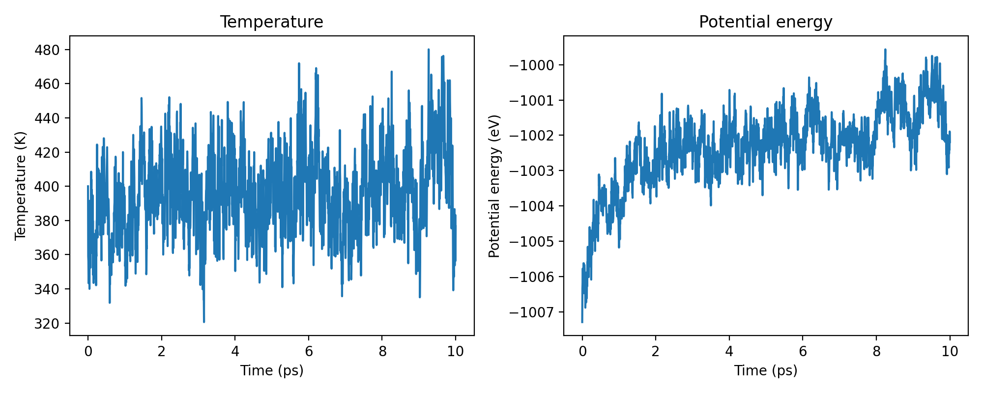
As a first sanity check we plot the temperature and potential energy along the trajectory: the thermostat should hold the temperature near its 400 K target (fluctuations are expected, given the small system). After a brief equilibration the potential energy should settle around a stable mean, with no long-term drift.

water_thermo = np.loadtxt("water_thermo.out", skiprows=1)
# columns: step temp pe etotal press vol
time_ps = water_thermo[:, 0] * 0.0005  # step × dt (0.5 fs) in ps

fig, axes = plt.subplots(1, 2, figsize=(10, 4), dpi=200)
axes[0].plot(time_ps, water_thermo[:, 1])
axes[0].set(xlabel="Time (ps)", ylabel="Temperature (K)", title="Temperature")
axes[1].plot(time_ps, water_thermo[:, 2])
axes[1].set(
    xlabel="Time (ps)", ylabel="Potential energy (eV)", title="Potential energy"
)
fig.tight_layout()
plt.show()

We can also inspect the trajectory interactively. Water molecules diffuse and the hydrogen-bond network continuously rearranges.

water_traj = ase.io.read("water_traj.lammpstrj", ":", format="lammps-dump-text")
for frame in water_traj:
    frame.wrap()
chemiscope.show(
    structures=water_traj,
    mode="structure",
    settings=chemiscope.quick_settings(
        trajectory=True,
        structure_settings={"playbackDelay": 20, "unitCell": True},
    ),
)

×

×

Adding ions: NaCl in water

PET-MAD can handle in principle any stable chemical element. We start by dissolving two NaCl units (two Na⁺ and two Cl⁻ ions) in 60 water molecules, a roughly 1.8 M solution. The only change to the LAMMPS input is the element map: the pair_coeff line now also assigns Na (Z=11) and Cl (Z=17). No new parameters and no retraining are involved: the same weights describe ion-water and ion-ion interactions out of the box.

# NaCl aqueous solution NVT at 400 K with PET-MAD-xs
# Atom types: 1=H, 2=O, 3=Na, 4=Cl

units metal
atom_style atomic

variable seed       index 23456
variable t_target   equal 400.0
variable tdamp      equal 100*dt
variable nsteps     equal 500         # 2000 * 0.5 fs = 1 ps
variable dump_every equal 10

read_data data/nacl.data

pair_style metatomic pet-mad-xs-v1.5.0.pt device cpu
pair_coeff * * 1 8 11 17

timestep 0.0005

neighbor 2.0 bin
neigh_modify one 50000 page 500000

thermo_style custom step temp pe etotal press vol
thermo 10

velocity all create ${t_target} ${seed} mom yes rot yes dist gaussian
reset_timestep 0

fix nve_int   all nve
fix thermostat all temp/csvr ${t_target} ${t_target} ${tdamp} ${seed}

print "step temp pe etotal press vol" file nacl_thermo.out
fix thermofile all print ${dump_every} "$(step) $(temp) $(pe) $(etotal) $(press) $(vol)" append nacl_thermo.out

dump traj all custom ${dump_every} nacl_traj.lammpstrj id type element xu yu zu
dump_modify traj element H O Na Cl sort id

run ${nsteps}

lmp -in in_nacl_nvt.lmp

Does that hold up quantitatively? The standard structural probe of solvation is the ion-oxygen radial distribution function g(r): the density of water oxygens at a distance r from each ion, normalized to the bulk density. A tall first peak followed by a deep minimum is the fingerprint of a well-defined hydration shell, and that first minimum sets the shell radius.

nacl_traj = ase.io.read("nacl_traj.lammpstrj", ":", format="lammps-dump-text")
g_na = []
r_na = []
g_cl = []
r_cl = []
for frame in nacl_traj[::10]:
    g_na_, r_na_ = get_rdf(frame, 6.0, 100, elements=["Na", "O"])
    g_cl_, r_cl_ = get_rdf(frame, 6.0, 100, elements=["Cl", "O"])
    g_na.append(g_na_)
    r_na.append(r_na_)
    g_cl.append(g_cl_)
    r_cl.append(r_cl_)
g_na = np.array(g_na).mean(axis=0)
r_na = np.array(r_na).mean(axis=0)
g_cl = np.array(g_cl).mean(axis=0)
r_cl = np.array(r_cl).mean(axis=0)

fig, ax = plt.subplots(figsize=(7, 4), dpi=200)
ax.plot(r_na, g_na, color="tab:orange", label="Na⁺-O")
ax.plot(r_cl, g_cl, color="tab:green", label="Cl⁻-O")
ax.axvline(3.1, color="tab:orange", ls="--", lw=0.8)
ax.axvline(3.8, color="tab:green", ls="--", lw=0.8)
ax.set(xlabel="r (Å)", ylabel="g(r)", title="Ion-oxygen radial distribution")
ax.legend()
plt.show()

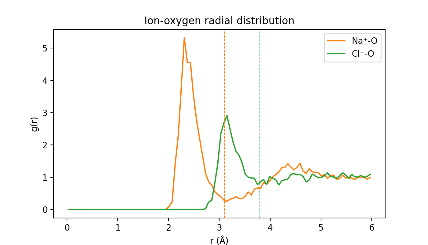
Both ions show a structured first peak and a clear first minimum (dashed lines, near 3.1 Å for Na⁺ and 3.8 Å for Cl⁻). Counting the water oxygens inside those radii every frame gives a coordination number, which we attach to the trajectory and show on the map beside the structure below. It fluctuates around 5-6 for Na⁺ and about 7 for Cl⁻ and never collapses: both shells survive the whole run. Drag the slider to follow structure and curve together, or use the map menu to switch between the two ions.

def first_shell_count(
    traj: list[ase.Atoms], ion: str, cutoff: float, other: str = "O"
) -> np.ndarray:
    """
    Mean number of other atoms within cutoff of each ion.

    :param traj: trajectory to analyze
    :param ion: element symbol of the ion (e.g. "Na" or "Cl")
    :param cutoff: shell radius in Å
    :param other: element symbol of the other species (default: "O")
    :return: array of shape (n_frames,) with the average count per ion at each frame
    """
    sym = np.array(traj[0].get_chemical_symbols())
    # L = traj[0].get_cell()[0, 0]
    i_ion = np.where(sym == ion)[0]
    i_other = np.where(sym == other)[0]
    counts = []
    for frame in traj:
        # pos = frame.get_positions()
        # d = pos[i_ion][:, None, :] - pos[i_other][None, :, :]
        # d -= np.round(d / L) * L  # minimum-image convention
        d = frame.get_all_distances(mic=True)[i_ion, :][:, i_other]
        counts.append((d < cutoff).sum(axis=1).mean())
    return np.array(counts)


n_na = first_shell_count(nacl_traj, "Na", 3.1)
n_cl = first_shell_count(nacl_traj, "Cl", 3.8)
time_ps = np.arange(len(nacl_traj)) * 0.0005 * 10  # 0.5 fs step, dumped every 10

for frame in nacl_traj:
    frame.wrap()
chemiscope.show(
    structures=nacl_traj,
    properties={
        "time [ps]": {"target": "structure", "values": time_ps},
        "Na+ first-shell waters": {"target": "structure", "values": n_na},
        "Cl- first-shell waters": {"target": "structure", "values": n_cl},
    },
    mode="default",
    settings=chemiscope.quick_settings(
        trajectory=True,
        x="time [ps]",
        y="Na+ first-shell waters",
        structure_settings={"playbackDelay": 20, "unitCell": True},
        map_settings={"markerOutline": False},
    ),
)

×

×

An organic mixture: ethanol-water

Ethanol (C₂H₅OH) adds a third element, carbon. For LAMMPS this is simply a third atom type, and the pair_coeff line grows by one entry to map C (Z=6). The model handles the new C-H, C-C, C-O and carbon-water interactions with no extra input. This kind of mixed organic/aqueous environment is common in chemistry, but can be tedious to parameterize with traditional force fields.

# Ethanol-water mixture NVT at 400 K with PET-MAD-xs
# Atom types: 1=H, 2=O, 3=C

units metal
atom_style atomic

variable seed       index 34567
variable t_target   equal 400.0
variable tdamp      equal 100*dt
variable nsteps     equal 500         # 2000 * 0.5 fs = 1 ps
variable dump_every equal 10

read_data data/ethanol_water.data

pair_style metatomic pet-mad-xs-v1.5.0.pt device cpu
pair_coeff * * 1 8 6

timestep 0.0005

neighbor 2.0 bin
neigh_modify one 50000 page 500000

thermo_style custom step temp pe etotal press vol
thermo 10

velocity all create ${t_target} ${seed} mom yes rot yes dist gaussian
reset_timestep 0

fix nve_int   all nve
fix thermostat all temp/csvr ${t_target} ${t_target} ${tdamp} ${seed}

print "step temp pe etotal press vol" file ethanol_thermo.out
fix thermofile all print ${dump_every} "$(step) $(temp) $(pe) $(etotal) $(press) $(vol)" append ethanol_thermo.out

dump traj all custom ${dump_every} ethanol_traj.lammpstrj id type element xu yu zu
dump_modify traj element H O C sort id

run ${nsteps}

lmp -in in_ethanol_nvt.lmp

We claimed that the two species mix and hydrogen-bond to each other; we can count those bonds explicitly. Using the standard geometric definition (an O-H…O motif with the two oxygens within 3.5 Å and an O-H…O angle above 150°) we classify each hydrogen bond as water-water or water-ethanol. (A hydroxyl H is identified as the H whose nearest heavy neighbor is an oxygen; an ethanol O is one bonded to a carbon.)

def count_hbonds(
    traj: list[ase.Atoms], r_oo: float = 3.5, angle: float = 150.0
) -> tuple[np.ndarray, np.ndarray]:
    """
    Per-frame counts of (water-water, water-ethanol) hydrogen bonds.

    :param traj: trajectory to analyze
    :param r_oo: O-O distance cutoff in Å
    :param angle: O-H...O angle cutoff in degrees
    :return: tuple of two arrays of shape (n_frames,) with the counts of water-water and
        water-ethanol H-bonds at each frame
    """
    sym = np.array(traj[0].get_chemical_symbols())
    L = traj[0].get_cell()[0, 0]
    iO = np.where(sym == "O")[0]
    iH = np.where(sym == "H")[0]
    iC = np.where(sym == "C")[0]
    heavy = np.concatenate([iO, iC])

    def mic(a, b):
        d = a[:, None, :] - b[None, :, :]
        return d - np.round(d / L) * L

    # ethanol oxygens have a carbon neighbor; topology is fixed, use the first frame
    p0 = traj[0].get_positions()
    eth_O = (np.linalg.norm(mic(p0[iO], p0[iC]), axis=-1) < 1.7).any(axis=1)
    cos_thr = np.cos(np.radians(angle))

    ww, we = [], []
    for frame in traj:
        p = frame.get_positions()
        # donor O-H pairs: each H whose nearest heavy neighbor is an oxygen
        dist_H = np.linalg.norm(mic(p[iH], p[heavy]), axis=-1)
        nn = np.argmin(dist_H, axis=1)
        is_oh = (nn < len(iO)) & (dist_H[np.arange(len(iH)), nn] < 1.3)
        Hd, Od = iH[is_oh], iO[nn[is_oh]]
        vHD = p[Od] - p[Hd]
        vHD -= np.round(vHD / L) * L  # H -> donor O
        vHA = -mic(p[Hd], p[iO])  # H -> every candidate acceptor O
        rDA = np.linalg.norm(mic(p[Od], p[iO]), axis=-1)  # donor O .. acceptor O
        nHD = np.linalg.norm(vHD, axis=-1)
        nHA = np.linalg.norm(vHA, axis=-1)
        cos = (vHD[:, None, :] * vHA).sum(-1) / (nHD[:, None] * nHA + 1e-9)
        hbond = (rDA < r_oo) & (cos < cos_thr)
        donor_eth = eth_O[nn[is_oh]][:, None]
        accpt_eth = eth_O[None, :]
        ww.append(int((hbond & ~donor_eth & ~accpt_eth).sum()))
        we.append(int((hbond & (donor_eth ^ accpt_eth)).sum()))
    return np.array(ww), np.array(we)


ethanol_traj = ase.io.read("ethanol_traj.lammpstrj", ":", format="lammps-dump-text")
hb_ww, hb_we = count_hbonds(ethanol_traj)
time_ps = np.arange(len(ethanol_traj)) * 0.0005 * 10

At every instant there are roughly a dozen water-ethanol hydrogen bonds (⟨n⟩ ≈ 12) and about forty water-water ones (⟨n⟩ ≈ 42), both steady across the run; ethanol-ethanol bonds are negligible at this dilution. That persistent water-ethanol count is the molecular signature of a miscible mixture: ethanol is not sequestered in a pocket but stitched into the water hydrogen-bond network. Both counts are attached to the trajectory below: scrub through it, or switch the map axis between the two curves.

for frame in ethanol_traj:
    frame.wrap()
chemiscope.show(
    structures=ethanol_traj,
    properties={
        "time [ps]": {"target": "structure", "values": time_ps},
        "water-ethanol H-bonds": {"target": "structure", "values": hb_we},
        "water-water H-bonds": {"target": "structure", "values": hb_ww},
    },
    mode="default",
    settings=chemiscope.quick_settings(
        trajectory=True,
        x="time [ps]",
        y="water-ethanol H-bonds",
        structure_settings={"playbackDelay": 20, "unitCell": True},
        map_settings={"markerOutline": False},
    ),
)

×

×

Extreme conditions: superionic water

The last system pushes far outside everyday chemistry. Deep inside the ice-giant planets (Uranus and Neptune) water is thought to exist in a superionic phase: the oxygen atoms stay locked on a crystalline lattice while the protons melt and diffuse through it like a liquid, turning the material into an ionic conductor. Reaching it requires roughly 3000 K and ~140 GPa. At these conditions common empirical water models are undefined, whereas an MLIP is reactive by construction.

We start from an ice-X-like configuration (a 4×4×4 supercell of a body-centered-cubic oxygen lattice, 128 water molecules) and hold it at 3000 K and fixed volume. Two settings change relative to the runs above: the temperature is much higher, and the timestep is shortened to 0.2 fs (timestep 0.0002) because atoms move much faster at 3000 K and the integration must stay stable.

# Superionic water NVT at 3000 K with PET-MAD-xs
# Pre-equilibrated at ~140 GPa; NVT keeps the volume fixed.
# Atom types: 1=H, 2=O

units metal
atom_style atomic

variable seed       index 45678
variable t_target   equal 3000.0
variable tdamp      equal 100*dt
variable nsteps     equal 50000        # 50000 * 0.2 fs = 10 ps
variable dump_every equal 25

read_data data/superionic_ice.data

pair_style metatomic pet-mad-xs-v1.5.1.pt device cpu
pair_coeff * * 1 8

timestep 0.0002                        # 0.2 fs (shorter for high-T/P stability)

neighbor 2.0 bin
neigh_modify one 50000 page 500000

thermo_style custom step temp pe etotal press vol
thermo 10

velocity all create ${t_target} ${seed} mom yes rot yes dist gaussian
reset_timestep 0

fix nve_int   all nve
fix thermostat all temp/csvr ${t_target} ${t_target} ${tdamp} ${seed}

print "step temp pe etotal press vol" file superionic_thermo.out
fix thermofile all print ${dump_every} "$(step) $(temp) $(pe) $(etotal) $(press) $(vol)" append superionic_thermo.out

dump traj all custom ${dump_every} superionic_traj.lammpstrj id type element xu yu zu
dump_modify traj element H O sort id

run ${nsteps}

lmp -in in_superionic_nvt.lmp

The clearest signature of the superionic phase is the mean-squared displacement (MSD) of each species. If the phase is truly superionic, the hydrogen MSD should grow linearly in time (Fickian diffusion, exactly as in a liquid) while the oxygen MSD stays small and flat, reflecting atoms that only rattle around fixed lattice sites.

Because the trajectory was dumped with unwrapped coordinates, the MSD is a plain average of squared displacements, with no periodic-boundary correction needed:

def compute_msd(traj: list, species: str) -> np.ndarray:
    symbols = np.array(traj[0].get_chemical_symbols())
    mask = symbols == species
    pos = np.array([f.get_positions()[mask] for f in traj])
    return np.mean(np.sum((pos - pos[0][np.newaxis]) ** 2, axis=-1), axis=-1)


sup_traj = ase.io.read("superionic_traj.lammpstrj", ":", format="lammps-dump-text")

dt_ps = 0.0002  # timestep in ps (0.2 fs)
dump_every = 25
time_ps = np.arange(len(sup_traj)) * dt_ps * dump_every

msd_H = compute_msd(sup_traj, "H")
msd_O = compute_msd(sup_traj, "O")

fig, ax = plt.subplots(figsize=(7, 4), dpi=200)
ax.plot(time_ps, msd_H, label="H")
ax.plot(time_ps, msd_O, label="O")
ax.set(
    xlabel="Time (ps)",
    ylabel="MSD (Ų)",
    title="Superionic water (3000 K, ~140 GPa)",
)
ax.legend()
plt.show()

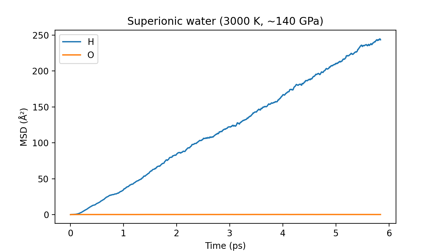
The two curves behave just as predicted: hydrogen diffuses freely while oxygen stays put. To watch the transition itself, we ramp the temperature from 300 K to 3000 K over a single trajectory. The input is the one above with a single change: the thermostat target sweeps from 300 K to 3000 K instead of being held fixed (fix temp/csvr 300 3000 ...). Run it with:

lmp -in in_superionic_ramp.lmp

While visualizing the trajectory, notice how the oxygen lattice stays ordered while the hydrogen atoms progressively diffuse and begin to flow between sites.

sup_ramp_traj = ase.io.read(
    "superionic_ramp_traj.lammpstrj", ":", format="lammps-dump-text"
)
sup_ramp_thermo = np.loadtxt("superionic_ramp_thermo.out", skiprows=1)
ramp_time_ps = sup_ramp_thermo[:, 0] * 0.0002
ramp_temp_K = sup_ramp_thermo[:, 1]

chemiscope.show(
    structures=sup_ramp_traj,
    properties={
        "time [ps]": {"target": "structure", "values": ramp_time_ps},
        "temperature [K]": {"target": "structure", "values": ramp_temp_K},
    },
    mode="default",
    settings=chemiscope.quick_settings(
        trajectory=True,
        x="time [ps]",
        y="temperature [K]",
        structure_settings={"playbackDelay": 5, "unitCell": True},
        map_settings={"markerOutline": False},
    ),
)

×

×

Where to go next

Throughout this recipe we used a foundational model out of the box, changing only the system and never the potential. That is often enough for a qualitative picture, a starting structure, or a screening study. For quantitative accuracy at a specific thermodynamic state, though, one often needs fine-tuning: a small, targeted set of DFT calculations specializes the universal model to the system or conditions of interest, at a fraction of the cost of training from scratch.

To go further:

• PET-MAD tutorial—how to set up and run PET-MAD yourself with ASE, i-PI and LAMMPS, for a diverse array of applications.

• Fine-tuning PET-MAD—how to specialize a foundational model to a target system for production-quality accuracy.

• Mendeleev’s nano-soup—the same model pushed to the limit: sampling a 102-element nanoparticle with replica-exchange MD and Monte Carlo atom swaps.